# library(tidyverse)
library(ggplot2)
library(vegan)
library(phyloseq)
# library (ape)
library(RColorBrewer)
Loading required package: permute
Loading required package: lattice
This is vegan 2.5-4
otu <- as.matrix(read.table("ASVs_counts.tsv", header=T, row.names=1)) #tabla de OTUs sin singletons, formato tabular.  eliminados con: http://qiime.org/scripts/filter_otus_from_otu_table.html
OTU = otu_table(otu, taxa_are_rows=T)
head(OTU)
taximat = as.matrix(read.table("ASVs_taxonomy.tsv", header=T, row.names=1)) #revisar los encabezados
taxi=tax_table(taximat)
metro = phyloseq(OTU, taxi)
sample_names(metro)
data= read.table("THEmetadata.txt", header=T, row.names=1, sep="\t")#los metadatos deben de estar en el mismo orden en el que estan en la tabla de OTUs:  sample_data(camaron)
sampledata = sample_data(data.frame(id=data$id, sample_location=data$sample_location, sample_id=data$sample_id,line_number=data$line_number, sample_type=data$sample_type, date=data$date, time=data$time, temperature_C=data$temperature_C, Humidity=data$Humidity, length_underground=data$ length_underground, length_superficial=data$length_superficial, length_elevated=data$length_elevated, length_total=data$length_total, elevation=data$elevation, station=data$station_hubs, train_track=data$train_track, train_notes=data$train_notes, station_notes=data$station_notes, geographical_zone=data$geographical_zone, weather=data$weather, stations_number=data$stations_number, latitude=data$latitude, longitude=data$longitude, people_affluence=data$people_affluence, Observed=data$Observed, Chao1=data$Chao1, Shannon=data$Shannon, Simpson=data$Simpson, row.names=sample_names(metro)))
# tree <- read.newick("metro.tre")
# tree <- collapse.singles(tree)
metro = phyloseq (OTU, sampledata, taxi)

metro
| <th scope=col>AM01</th><th scope=col>AM02</th><th scope=col>AM03</th><th scope=col>AM04</th><th scope=col>AM05</th><th scope=col>AM06</th><th scope=col>AM07</th><th scope=col>AM08</th><th scope=col>AM09</th><th scope=col>AM10</th><th scope=col>⋯</th><th scope=col>AM39</th><th scope=col>AM40</th><th scope=col>AM41</th><th scope=col>AM42</th><th scope=col>AM43</th><th scope=col>AM44</th><th scope=col>AM45</th><th scope=col>AM46</th><th scope=col>AM47</th><th scope=col>AM48</th> | ||||||||||||||||||||
|---|---|---|---|---|---|---|---|---|---|---|---|---|---|---|---|---|---|---|---|---|
| 10459 | 8198 | 6740 | 5339 | 114 | 15981 | 9607 | 4123 | 5860 | 4780 | ⋯ | 9224 | 20148 | 15588 | 15573 | 7217 | 43753 | 19733 | 13121 | 35807 | 19170 |
| 2232 | 6735 | 3194 | 2244 | 69 | 3268 | 3663 | 1786 | 2574 | 3542 | ⋯ | 1476 | 3016 | 3018 | 1699 | 764 | 1450 | 3853 | 2261 | 1191 | 2595 |
| 997 | 1372 | 3194 | 0 | 0 | 0 | 0 | 462 | 0 | 0 | ⋯ | 487 | 389 | 299 | 3555 | 1510 | 477 | 0 | 3658 | 502 | 0 |
| 705 | 1456 | 454 | 1279 | 115 | 485 | 5619 | 367 | 2370 | 786 | ⋯ | 1682 | 3666 | 1036 | 2506 | 474 | 6183 | 5043 | 737 | 2413 | 2674 |
| 1752 | 1938 | 1800 | 1050 | 31 | 7149 | 1617 | 1268 | 1337 | 2806 | ⋯ | 2826 | 639 | 1106 | 1322 | 685 | 1740 | 2532 | 2583 | 690 | 4561 |
| 1053 | 2408 | 672 | 3084 | 72 | 1809 | 3995 | 675 | 7260 | 1097 | ⋯ | 3187 | 1961 | 1231 | 791 | 430 | 983 | 5016 | 1659 | 305 | 1469 |
<ol class=list-inline> <li>‘AM01’</li> <li>‘AM02’</li> <li>‘AM03’</li> <li>‘AM04’</li> <li>‘AM05’</li> <li>‘AM06’</li> <li>‘AM07’</li> <li>‘AM08’</li> <li>‘AM09’</li> <li>‘AM10’</li> <li>‘AM11’</li> <li>‘AM12’</li> <li>‘AM13’</li> <li>‘AM14’</li> <li>‘AM15’</li> <li>‘AM16’</li> <li>‘AM17’</li> <li>‘AM18’</li> <li>‘AM19’</li> <li>‘AM20’</li> <li>‘AM21’</li> <li>‘AM22’</li> <li>‘AM23’</li> <li>‘AM24’</li> <li>‘AM26’</li> <li>‘AM27’</li> <li>‘AM28’</li> <li>‘AM29’</li> <li>‘AM30’</li> <li>‘AM31’</li> <li>‘AM32’</li> <li>‘AM33’</li> <li>‘AM34’</li> <li>‘AM35’</li> <li>‘AM36’</li> <li>‘AM37’</li> <li>‘AM38’</li> <li>‘AM39’</li> <li>‘AM40’</li> <li>‘AM41’</li> <li>‘AM42’</li> <li>‘AM43’</li> <li>‘AM44’</li> <li>‘AM45’</li> <li>‘AM46’</li> <li>‘AM47’</li> <li>‘AM48’</li> </ol>
phyloseq-class experiment-level object
otu_table()   OTU Table:         [ 22673 taxa and 47 samples ]
sample_data() Sample Data:       [ 47 samples by 28 sample variables ]
tax_table()   Taxonomy Table:    [ 22673 taxa by 6 taxonomic ranks ]
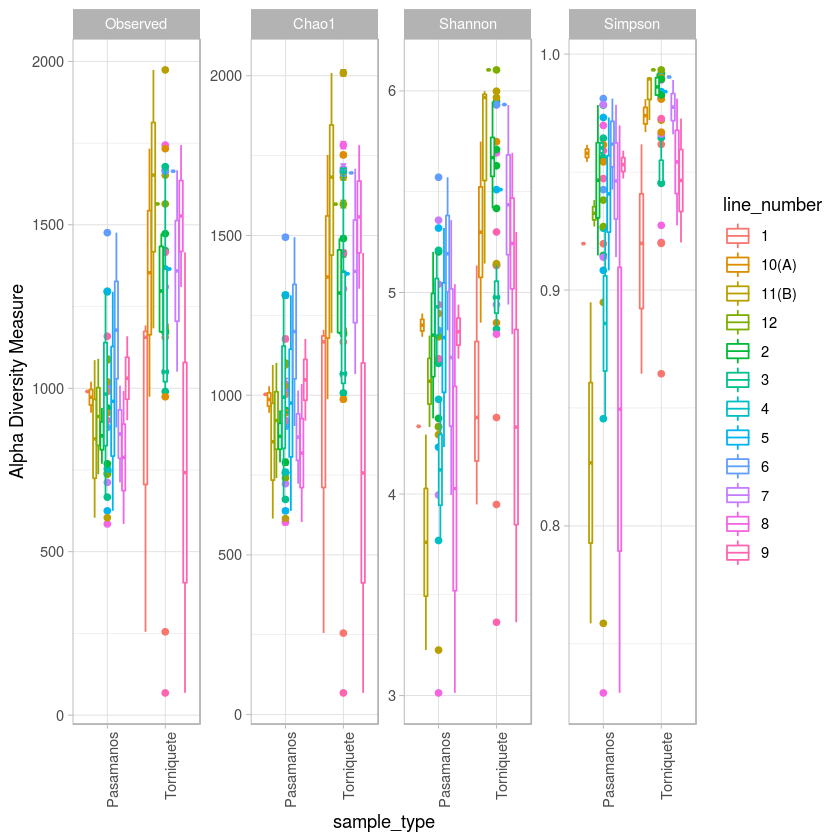
p <- plot_richness(metro, x="sample_type", color="line_number", measures=c("Observed", "Chao1", "Shannon", "Simpson")) + geom_boxplot()+theme_light() + theme(axis.text.x=element_text(angle=90, hjust=1))
#p$data
a <-p$data
p
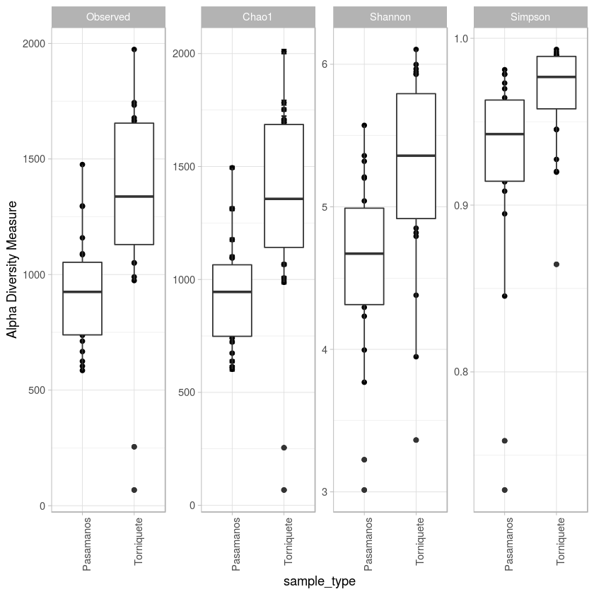
p <- plot_richness(metro, x="sample_type", measures=c("Observed", "Chao1", "Shannon", "Simpson")) + geom_boxplot()+theme_light() + theme(axis.text.x=element_text(angle=90, hjust=1))
#p$data
p
ggsave("histogramaASV_Alfa_diversidad.pdf")
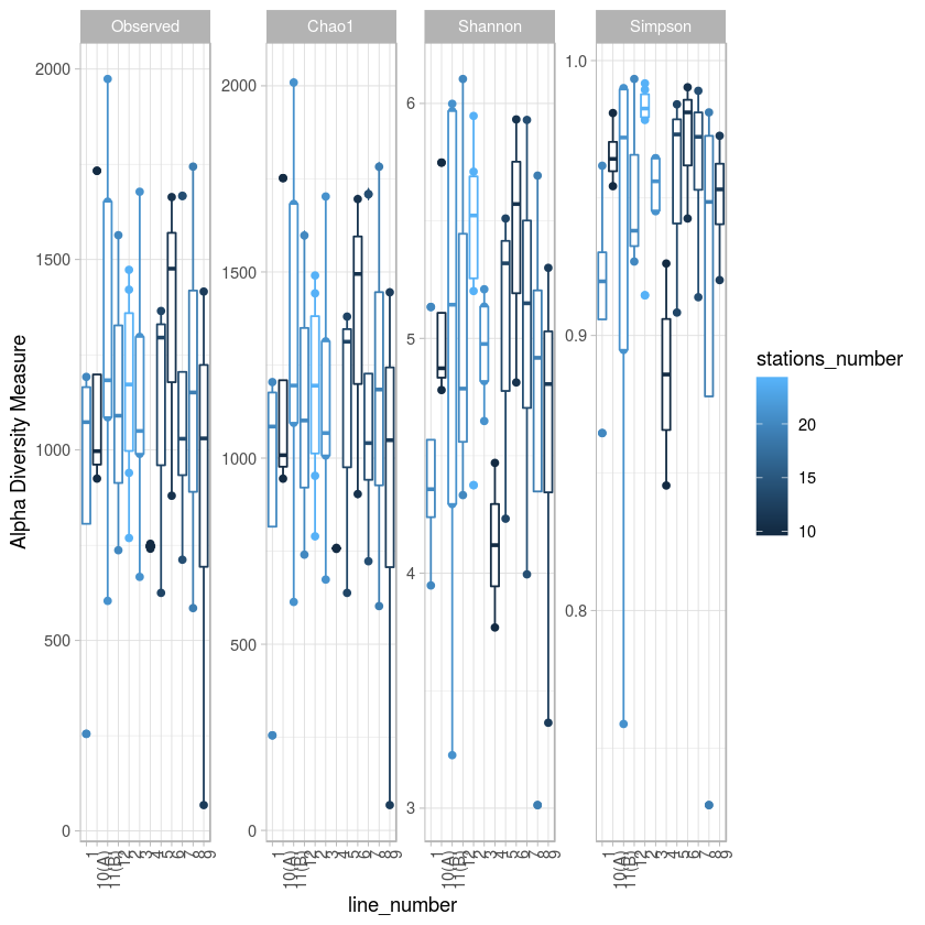
p <- plot_richness(metro, x="line_number", color="stations_number", measures=c("Observed", "Chao1", "Shannon", "Simpson")) + geom_boxplot()+theme_light() + theme(axis.text.x=element_text(angle=90, hjust=1))
#p$data
p
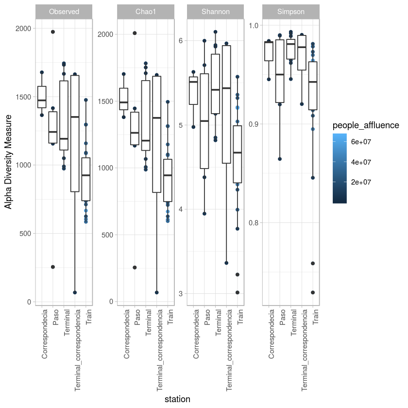
p <- plot_richness(metro, x="station",color="people_affluence", measures=c("Observed", "Chao1", "Shannon", "Simpson")) + geom_boxplot()+theme_light() + theme(axis.text.x=element_text(angle=90, hjust=1))
#p$data
p
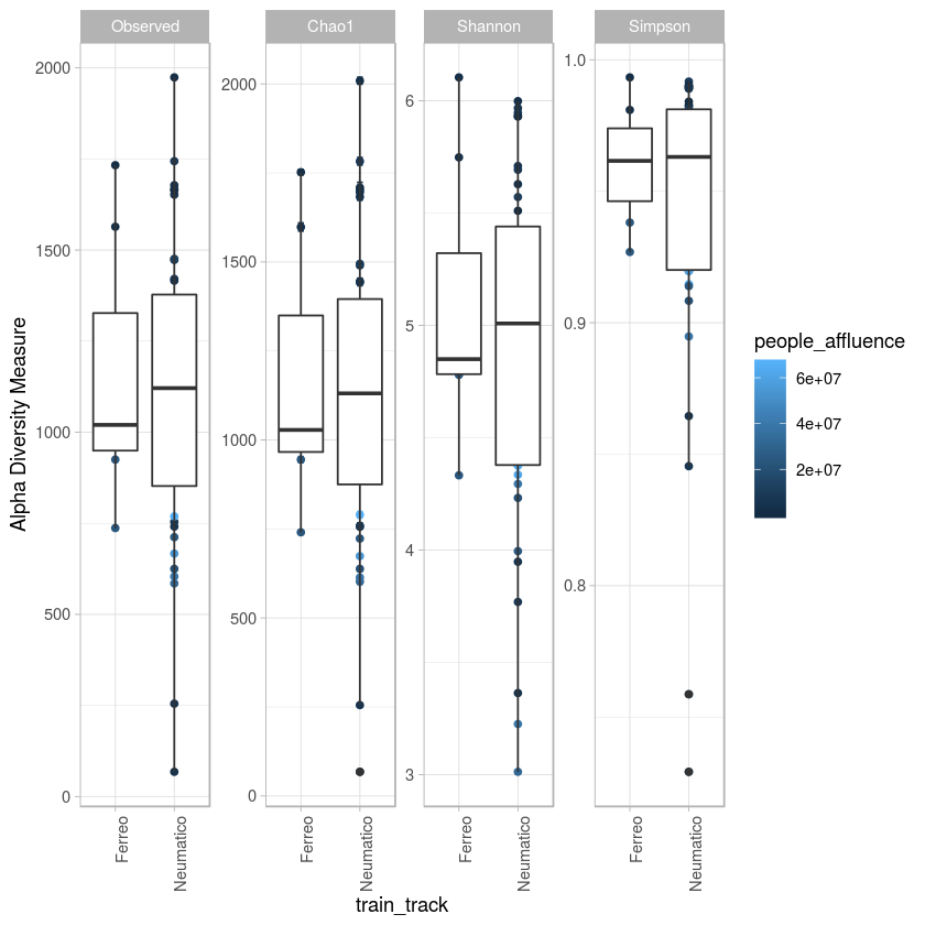
p <- plot_richness(metro, x="train_track",color="people_affluence", measures=c("Observed", "Chao1", "Shannon", "Simpson")) + geom_boxplot()+theme_light() + theme(axis.text.x=element_text(angle=90, hjust=1))
#p$data
p
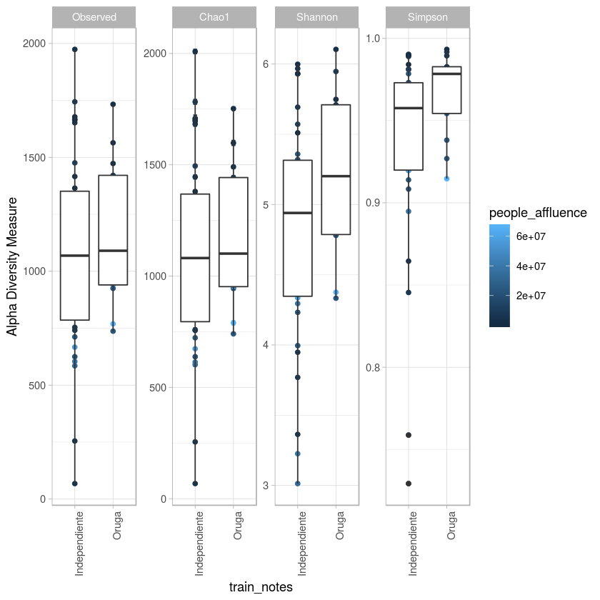
p <- plot_richness(metro, x="train_notes",color="people_affluence", measures=c("Observed", "Chao1", "Shannon", "Simpson")) + geom_boxplot()+theme_light() + theme(axis.text.x=element_text(angle=90, hjust=1))
#p$data
p
p <- plot_richness(metro, x="station_notes",color="people_affluence", measures=c("Observed", "Chao1", "Shannon", "Simpson")) + geom_boxplot()+theme_light() + theme(axis.text.x=element_text(angle=90, hjust=1))
#p$data
# p
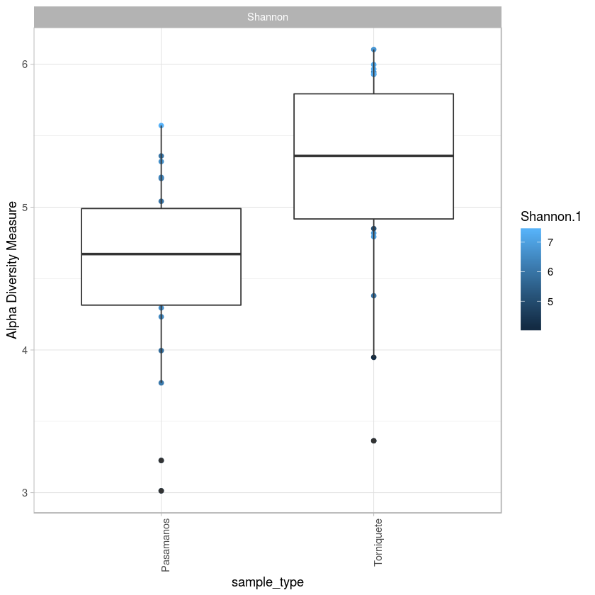
p <- plot_richness(metro, x="sample_type",color="Shannon.1", measures= "Shannon") + geom_boxplot()+theme_light() + theme(axis.text.x=element_text(angle=90, hjust=1))
a<- p$data
summary
p
write.csv(a,"shannon.estacion.csv",sep="\t")
                      id                  sample_location   sample_id
 Barranca_del_muerto_7 :  4   Train               :92     AM01   :  4
 Buenavista_B          :  4   Barranca_del_muerto : 4     AM02   :  4
 Chilpancingo_9        :  4   Buenavista          : 4     AM03   :  4
 Ciudad_Azteca_B       :  4   Chilpancingo        : 4     AM04   :  4
 Constitucion_de_1917_8:  4   Ciudad_Azteca       : 4     AM05   :  4
 Cuatro_caminos_2      :  4   Constitucion_de_1917: 4     AM06   :  4
 (Other)               :164   (Other)             :76     (Other):164
  line_number     sample_type      date             time     temperature_C
 2      :24   Pasamanos :92   2/5/16 :36   11:25:00 AM:  8   Min.   :25.90
 11(B)  :20   Torniquete:96   3/5/16 :28   11:42:00 AM:  8   1st Qu.:29.10
 3      :20                   4/16/27:36   1:20:00 PM :  8   Median :30.40
 1      :16                   4/16/28:24   12:05:00 PM:  8   Mean   :30.15
 10(A)  :16                   4/16/29:40   12:40:00 PM:  8   3rd Qu.:31.30
 7      :16                   4/5/16 :24   12:50:00 PM:  8   Max.   :33.30
 (Other):76                                (Other)    :140
    Humidity     length_underground length_superficial length_elevated
 Min.   :25.00   Min.   : 0.00      Min.   : 0.000     Min.   : 0.000
 1st Qu.:27.00   1st Qu.: 5.38      1st Qu.: 0.000     1st Qu.: 0.000
 Median :30.00   Median :11.86      Median : 4.449     Median : 0.000
 Mean   :30.38   Mean   :11.05      Mean   : 5.485     Mean   : 2.001
 3rd Qu.:32.00   3rd Qu.:16.79      3rd Qu.:10.724     3rd Qu.: 4.185
 Max.   :41.00   Max.   :18.14      Max.   :15.151     Max.   :11.533

  length_total     elevation                        station      train_track
 Min.   :11.00   Min.   :2231   Correspondecia          :12   Ferreo   : 28
 1st Qu.:16.00   1st Qu.:2237   Paso                    :24   Neumatico:160
 Median :18.00   Median :2242   Terminal                :44
 Mean   :18.83   Mean   :2250   Terminal_correspondencia:16
 3rd Qu.:22.00   3rd Qu.:2256   Train                   :92
 Max.   :25.00   Max.   :2303
                 NA's   :92
        train_notes            station_notes geographical_zone weather
 Independiente:136   Cajon_subterraneo:44    Centro  :20       B1  :16
 Oruga        : 52   Elevada          :36    Norte   :28       C1  :64
                     Superficial      :12    Oriente :20       C2  :16
                     Tunel            : 4    Poniente:12       NA's:92
                     NA's             :92    Sur     :16
                                             NA's    :92

 stations_number    latitude       longitude      people_affluence
 Min.   :10.00   Min.   :19.29   Min.   :-99.22   Min.   :  499350
 1st Qu.:12.00   1st Qu.:19.39   1st Qu.:-99.17   1st Qu.: 4190568
 Median :19.00   Median :19.43   Median :-99.14   Median : 9523016
 Mean   :17.15   Mean   :19.43   Mean   :-99.13   Mean   :17859153
 3rd Qu.:21.00   3rd Qu.:19.49   3rd Qu.:-99.10   3rd Qu.:24196452
 Max.   :24.00   Max.   :19.53   Max.   :-98.96   Max.   :66232325
                 NA's   :92      NA's   :92
   Observed.1       Chao1.1          Shannon.1       Simpson.1
 Min.   :  428   Min.   :  840.2   Min.   :4.102   Min.   :0.8984
 1st Qu.: 7655   1st Qu.:12618.1   1st Qu.:6.004   1st Qu.:0.9802
 Median :10129   Median :15375.8   Median :6.410   Median :0.9872
 Mean   : 9904   Mean   :15141.1   Mean   :6.380   Mean   :0.9827
 3rd Qu.:12677   3rd Qu.:18521.1   3rd Qu.:6.863   3rd Qu.:0.9916
 Max.   :16179   Max.   :23052.1   Max.   :7.384   Max.   :0.9960

   samples              variable      value                 se
 Length:188         Observed:47   Min.   :   0.7292   Min.   : 0.000
 Class :character   Chao1   :47   1st Qu.:   2.5084   1st Qu.: 5.580
 Mode  :character   Shannon :47   Median :  37.0522   Median : 7.086
                    Simpson :47   Mean   : 561.0525   Mean   : 6.989
                                  3rd Qu.:1087.0000   3rd Qu.: 8.543
                                  Max.   :2009.0065   Max.   :17.183
                                                      NA's   :141


Warning message:
“Removed 141 rows containing missing values (geom_errorbar).”Warning message:
“Removed 141 rows containing missing values (geom_errorbar).”
Saving 6.67 x 6.67 in image
Warning message:
“Removed 141 rows containing missing values (geom_errorbar).”Warning message:
“Removed 141 rows containing missing values (geom_errorbar).”
Warning message:
“Removed 141 rows containing missing values (geom_errorbar).”
Warning message:
“Removed 141 rows containing missing values (geom_errorbar).”
Warning message:
“Removed 141 rows containing missing values (geom_errorbar).”
Warning message in write.csv(a, "shannon.estacion.csv", sep = "\t"):
“attempt to set 'sep' ignored”
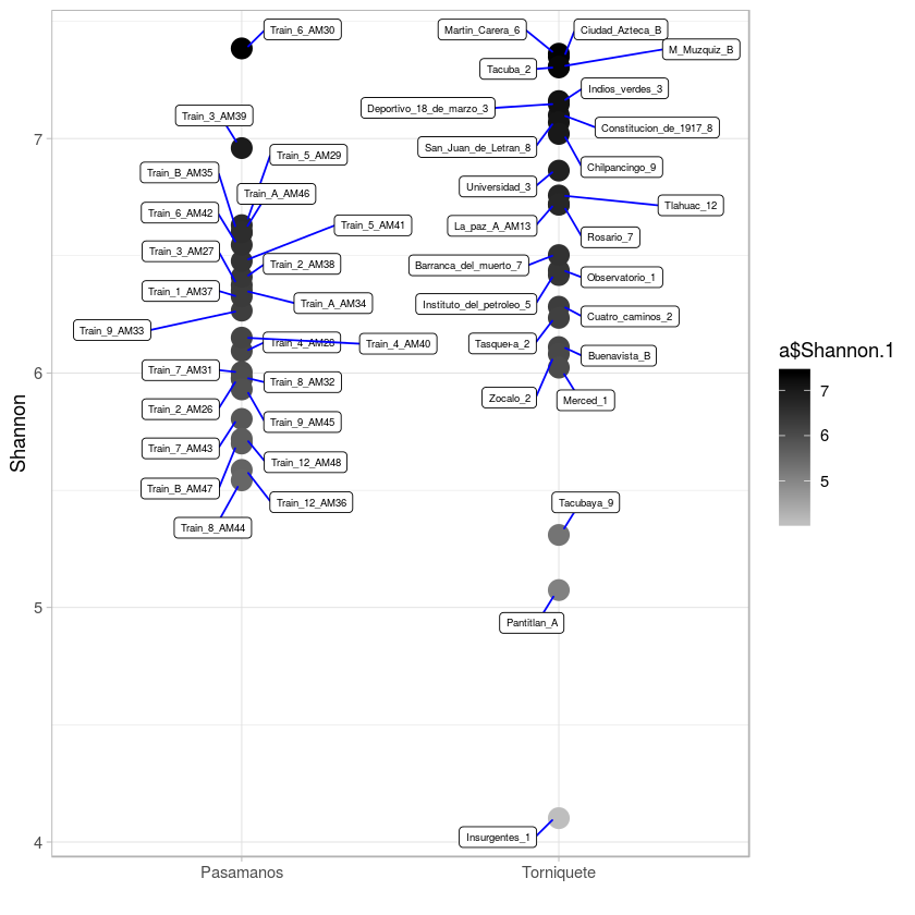
library(ggrepel)
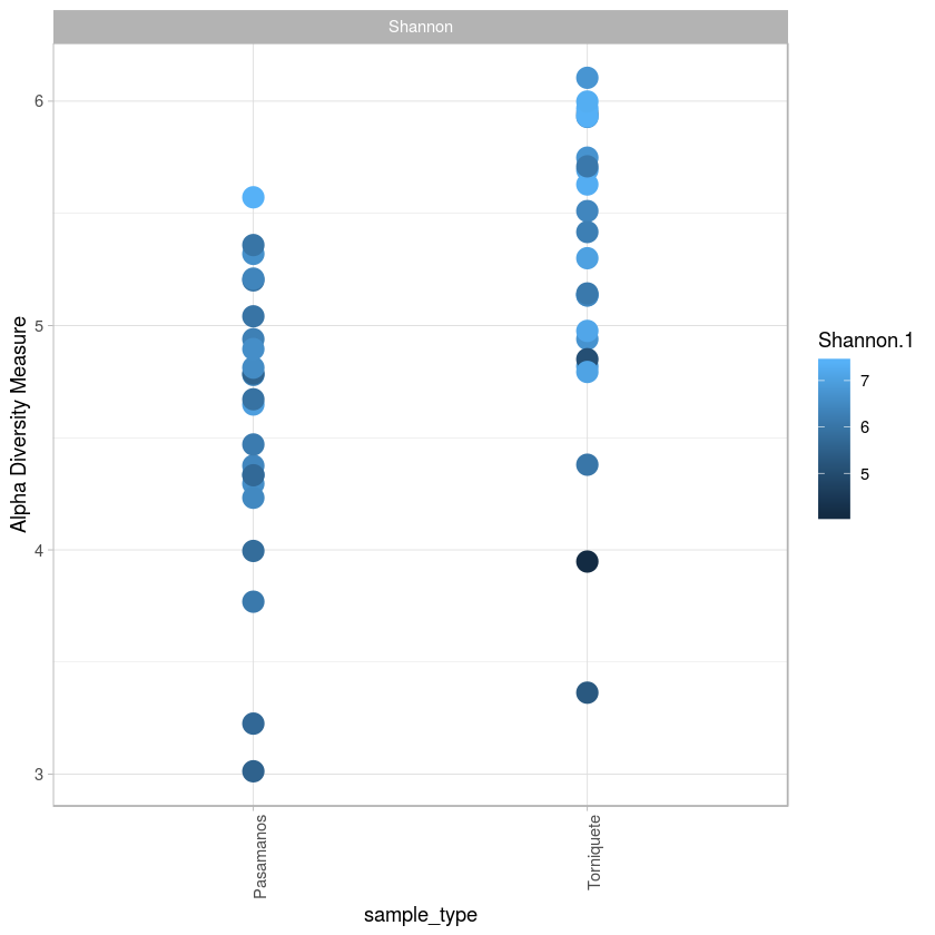
p <- plot_richness(metro, x="sample_type",color="Shannon.1", measures= "Shannon")
p + geom_point(size=5, alpha=1) + scale_fill_gradient(low="#F1E8FA", high="#FA7500", na.value = "white") + theme_light() + theme(axis.text.x=element_text(angle=90, hjust=1))
a<-as.data.frame(p$data)
head(a)
# head(p$data$id)
# head(a)
shannonplot <- ggplot(a, aes(x=a$sample_type, y=(a$Shannon.1))) + geom_point(aes(colour=a$Shannon.1), size=5) + scale_colour_gradient(low="#bebebe", high="#000000", na.value = "white")+ theme_light() +
# geom_text(aes(label=a$id), hjust=-0.1, vjust=0, size=2) +
xlab("") + ylab("Shannon")
shannonplot + geom_label_repel(aes(label = a$id),
box.padding = 0.35,
point.padding = 0.5,
segment.color = 'blue', size=2)
# ggplot(data=yx, aes(x = yx$orden, y= reorder(Genus, Abundance), fill= Abundance)) +
# geom_raster() + theme_minimal () +
# xlab("") + ylab("") +
# scale_fill_gradient(low="#bebebe", high="#000000", na.value = "white", trans = "log10") +
# theme(axis.text.x = element_text( angle = 90, hjust = 1),
# axis.text.y = element_text(size = 4))
# write.csv(a,"shannon.estacion.csv",sep="\t")
# library(ggplot2)
# library(ggrepel)
# nba <- read.csv("http://datasets.flowingdata.com/ppg2008.csv", sep = ",")
# nbaplot <- ggplot(nba, aes(x= MIN, y = PTS)) +
# geom_point(color = "blue", size = 3)
# ### geom_label_repel
# nbaplot +
# geom_label_repel(aes(label = Name),
# box.padding = 0.35,
# point.padding = 0.5,
# segment.color = 'grey50') +
# theme_classic()
| Indios_verdes_3 | Indios_verdes | AM01 | 3 | Torniquete | 2/5/16 | 2:23:00 PM | 30.4 | 27 | 18.145 | ⋯ | -99.11940 | 10176457 | 12677 | 19699.2193 | 7.160039 | 0.9921556 | AM01 | Shannon | 5.135283 | NA |
| Instituto_del_petroleo_5 | Instituto_del_petroleo | AM02 | 5 | Torniquete | 4/16/29 | 1:17:00 PM | 28.3 | 30 | 4.951 | ⋯ | -99.14480 | 499350 | 10722 | 16496.3811 | 6.417885 | 0.9890120 | AM02 | Shannon | 5.510396 | NA |
| Rosario_7 | Rosario | AM03 | 7 | Torniquete | 4/16/29 | 12:40:00 PM | 29.2 | 29 | 17.754 | ⋯ | -99.17970 | 3220719 | 11986 | 18521.1304 | 6.718174 | 0.9892510 | AM03 | Shannon | 4.939963 | NA |
| Cuatro_caminos_2 | Cuatro_caminos | AM04 | 2 | Torniquete | 4/16/29 | 11:42:00 AM | 30.3 | 30 | 12.550 | ⋯ | -99.21550 | 9523016 | 5425 | 8341.2612 | 6.283001 | 0.9939737 | AM04 | Shannon | 5.946868 | NA |
| Tacubaya_9 | Tacubaya | AM05 | 9 | Torniquete | 4/16/27 | 1:41:00 PM | 30.4 | 26 | 9.531 | ⋯ | -99.18830 | 4190568 | 428 | 840.2462 | 5.309640 | 0.9899266 | AM05 | Shannon | 3.363853 | NA |
| Observatorio_1 | Observatorio | AM06 | 1 | Torniquete | 4/5/16 | 2:35:00 PM | 32.2 | 28 | 16.786 | ⋯ | -99.19978 | 6489055 | 10523 | 17035.5115 | 6.437592 | 0.9859032 | AM06 | Shannon | 5.133815 | NA |
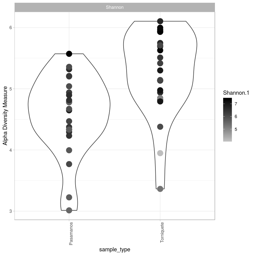
library(ggrepel)
p <- plot_richness(metro, x="sample_type",color="Shannon.1", measures= "Shannon")
p + geom_violin()+ geom_point(aes(colour=a$Shannon.1),size=5, alpha=1) + scale_colour_gradient(low="#bebebe", high="#000000", na.value = "white") + theme_light() + theme(axis.text.x=element_text(angle=90, hjust=1))
library(dplyr)
p <- plot_richness(metro, measures=c("Observed", "Chao1", "Shannon", "Simpson")) + geom_boxplot()+theme_light() + theme(axis.text.x=element_text(angle=90, hjust=1))
#p$data
#a <-p$data
#summary(a)
#write.table(a, "data.csv") Se edita para dejar en el formato id Observed Chao1 Shannon Simpson
meta <- read.table("THEmetadata.txt",sep="\t",header=T,row.names = 1) #data.csv se hizo a partir de la tabla anterior para calcular
#los datos de diversidad alfa
head(meta)
summary(meta)
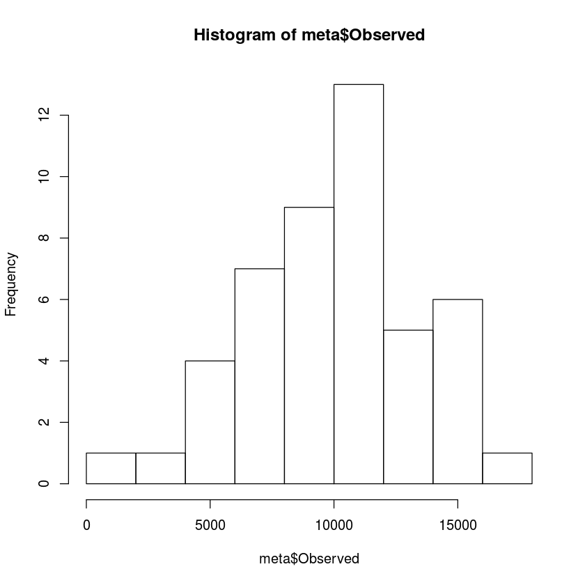
hist(meta$Observed, breaks=10)
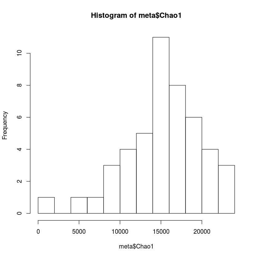
hist(meta$Chao1, breaks=10)
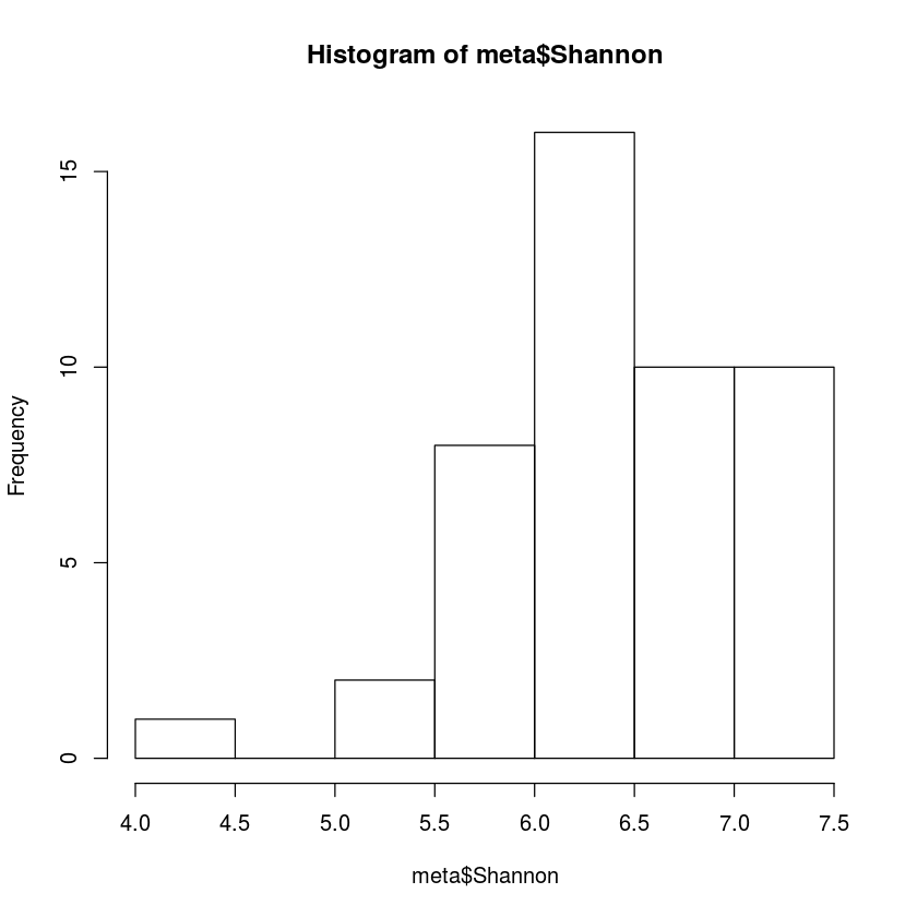
hist(meta$Shannon, breaks=10)
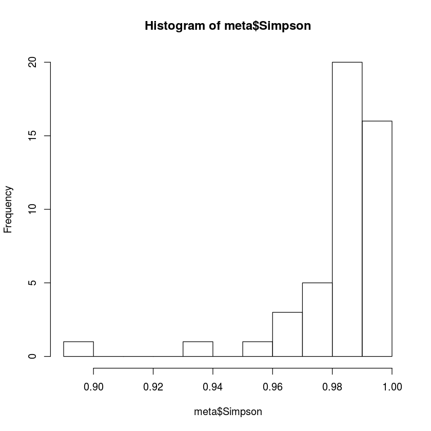
hist(meta$Simpson, breaks=10)
| <th scope=col>otu</th><th scope=col>id</th><th scope=col>sample_location</th><th scope=col>sample_id</th><th scope=col>line_number</th><th scope=col>sample_type</th><th scope=col>date</th><th scope=col>time</th><th scope=col>temperature_C</th><th scope=col>Humidity</th><th scope=col>⋯</th><th scope=col>geographical_zone</th><th scope=col>weather</th><th scope=col>stations_number</th><th scope=col>latitude</th><th scope=col>longitude</th><th scope=col>people_affluence</th><th scope=col>Observed</th><th scope=col>Chao1</th><th scope=col>Shannon</th><th scope=col>Simpson</th> | ||||||||||||||||||||
|---|---|---|---|---|---|---|---|---|---|---|---|---|---|---|---|---|---|---|---|---|
| Indios_verdes_3 | Indios_verdes_3 | Indios_verdes | AM01 | 3 | Torniquete | 2/5/16 | 2:23:00 PM | 30.4 | 27 | ⋯ | Norte | C1 | 21 | 19.4955 | -99.11940 | 10176457 | 12677 | 19699.2193 | 7.160039 | 0.9921556 |
| Instituto_del_petroleo_5 | Instituto_del_petroleo_5 | Instituto_del_petroleo | AM02 | 5 | Torniquete | 4/16/29 | 1:17:00 PM | 28.3 | 30 | ⋯ | Norte | C1 | 13 | 19.4890 | -99.14480 | 499350 | 10722 | 16496.3811 | 6.417885 | 0.9890120 |
| Rosario_7 | Rosario_7 | Rosario | AM03 | 7 | Torniquete | 4/16/29 | 12:40:00 PM | 29.2 | 29 | ⋯ | Norte | C1 | 14 | 19.5050 | -99.17970 | 3220719 | 11986 | 18521.1304 | 6.718174 | 0.9892510 |
| Cuatro_caminos_2 | Cuatro_caminos_2 | Cuatro_caminos | AM04 | 2 | Torniquete | 4/16/29 | 11:42:00 AM | 30.3 | 30 | ⋯ | Poniente | C2 | 24 | 19.4606 | -99.21550 | 9523016 | 5425 | 8341.2612 | 6.283001 | 0.9939737 |
| Tacubaya_9 | Tacubaya_9 | Tacubaya | AM05 | 9 | Torniquete | 4/16/27 | 1:41:00 PM | 30.4 | 26 | ⋯ | Poniente | C1 | 12 | 19.4024 | -99.18830 | 4190568 | 428 | 840.2462 | 5.309640 | 0.9899266 |
| Observatorio_1 | Observatorio_1 | Observatorio | AM06 | 1 | Torniquete | 4/5/16 | 2:35:00 PM | 32.2 | 28 | ⋯ | Poniente | C2 | 20 | 19.3985 | -99.19978 | 6489055 | 10523 | 17035.5115 | 6.437592 | 0.9859032 |
                     otu                          id
 Barranca_del_muerto_7 : 1   Barranca_del_muerto_7 : 1
 Buenavista_B          : 1   Buenavista_B          : 1
 Chilpancingo_9        : 1   Chilpancingo_9        : 1
 Ciudad_Azteca_B       : 1   Ciudad_Azteca_B       : 1
 Constitucion_de_1917_8: 1   Constitucion_de_1917_8: 1
 Cuatro_caminos_2      : 1   Cuatro_caminos_2      : 1
 (Other)               :41   (Other)               :41
             sample_location   sample_id   line_number     sample_type
 Train               :23     AM01   : 1   2      : 6   Pasamanos :23
 Barranca_del_muerto : 1     AM02   : 1   11(B)  : 5   Torniquete:24
 Buenavista          : 1     AM03   : 1   3      : 5
 Chilpancingo        : 1     AM04   : 1   1      : 4
 Ciudad_Azteca       : 1     AM05   : 1   10(A)  : 4
 Constitucion_de_1917: 1     AM06   : 1   7      : 4
 (Other)             :19     (Other):41   (Other):19
      date             time    temperature_C      Humidity
 2/5/16 : 9   11:25:00 AM: 2   Min.   :25.90   Min.   :25.00
 3/5/16 : 7   11:42:00 AM: 2   1st Qu.:29.10   1st Qu.:27.00
 4/16/27: 9   1:20:00 PM : 2   Median :30.40   Median :30.00
 4/16/28: 6   12:05:00 PM: 2   Mean   :30.15   Mean   :30.38
 4/16/29:10   12:40:00 PM: 2   3rd Qu.:31.30   3rd Qu.:32.00
 4/5/16 : 6   12:50:00 PM: 2   Max.   :33.30   Max.   :41.00
              (Other)    :35
 length_underground length_superficial length_elevated   length_total
 Min.   : 0.00      Min.   : 0.000     Min.   : 0.000   Min.   :11.00
 1st Qu.: 5.38      1st Qu.: 0.000     1st Qu.: 0.000   1st Qu.:16.50
 Median :11.86      Median : 4.449     Median : 0.000   Median :18.00
 Mean   :11.05      Mean   : 5.485     Mean   : 2.001   Mean   :18.83
 3rd Qu.:16.79      3rd Qu.:10.090     3rd Qu.: 4.185   3rd Qu.:22.00
 Max.   :18.14      Max.   :15.151     Max.   :11.533   Max.   :25.00

   elevation                      station_hubs    train_track
 Min.   :2231   Correspondecia          : 3    Ferreo   : 7
 1st Qu.:2237   Paso                    : 6    Neumatico:40
 Median :2242   Terminal                :11
 Mean   :2250   Terminal_correspondencia: 4
 3rd Qu.:2256   Train                   :23
 Max.   :2303
 NA's   :23
        train_notes           station_notes geographical_zone weather
 Independiente:34   Cajon_subterraneo:11    Centro  : 5       B1  : 4
 Oruga        :13   Elevada          : 9    Norte   : 7       C1  :16
                    Superficial      : 3    Oriente : 5       C2  : 4
                    Tunel            : 1    Poniente: 3       NA's:23
                    NA's             :23    Sur     : 4
                                            NA's    :23

 stations_number    latitude       longitude      people_affluence
 Min.   :10.00   Min.   :19.29   Min.   :-99.22   Min.   :  499350
 1st Qu.:12.00   1st Qu.:19.39   1st Qu.:-99.17   1st Qu.: 4284103
 Median :19.00   Median :19.43   Median :-99.14   Median : 9523016
 Mean   :17.15   Mean   :19.43   Mean   :-99.13   Mean   :17859153
 3rd Qu.:21.00   3rd Qu.:19.49   3rd Qu.:-99.10   3rd Qu.:24196452
 Max.   :24.00   Max.   :19.53   Max.   :-98.96   Max.   :66232325
                 NA's   :23      NA's   :23
    Observed         Chao1            Shannon         Simpson
 Min.   :  428   Min.   :  840.2   Min.   :4.102   Min.   :0.8984
 1st Qu.: 7732   1st Qu.:12826.6   1st Qu.:6.014   1st Qu.:0.9813
 Median :10129   Median :15375.8   Median :6.410   Median :0.9872
 Mean   : 9904   Mean   :15141.1   Mean   :6.380   Mean   :0.9827
 3rd Qu.:12332   3rd Qu.:18371.5   3rd Qu.:6.810   3rd Qu.:0.9915
 Max.   :16179   Max.   :23052.1   Max.   :7.384   Max.   :0.9960
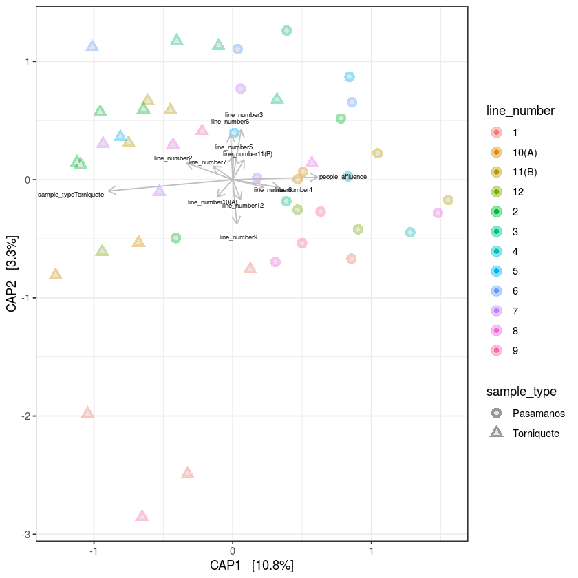
metroCAP.ORD <- ordinate(metro, "CAP", "bray", ~ people_affluence + line_number + sample_type)

metroCAP.ORD

cap_plot <- plot_ordination(metro, metroCAP.ORD, color="line_number", axes =c(1,2)) + aes(shape= sample_type) + geom_point(aes(colour = line_number), alpha=0.4, size=4) + geom_point(colour = "grey90", size=1.5) + theme_bw()


arrowmat <- vegan::scores(metroCAP.ORD, display="bp")
arrowdf <- data.frame(labels=rownames(arrowmat), arrowmat)

# Define the arrow aesthetic mapping

arrow_map <- aes(xend = CAP1,

    yend = CAP2,
    x = 0,
    y = 0,
    shape = NULL,
    color = NULL,
    label = labels)


label_map <- aes(x = 1.3 * CAP1,

    y = 1.3 * CAP2,
    shape = NULL,
    color = NULL,
    label = labels)


arrowhead = arrow(length = unit(0.02, "npc"))


cap_plot  +

  geom_segment(
    mapping = arrow_map,
    size = .5,
    data = arrowdf,
    color = "gray",
    arrow = arrowhead

  ) +

  geom_text(
    mapping = label_map,
    size = 2,
    data = arrowdf,
    show.legend = FALSE
  )


an <- anova(metroCAP.ORD, permutations=9999)
an
Call: capscale(formula = OTU ~ people_affluence + line_number +
sample_type, data = data, distance = distance)

              Inertia Proportion Rank
Total          9.2927     1.0000
Constrained    3.0265     0.3257   13
Unconstrained  6.2662     0.6743   33
Inertia is squared Bray distance
Species scores projected from ‘OTU’

Eigenvalues for constrained axes:
  CAP1   CAP2   CAP3   CAP4   CAP5   CAP6   CAP7   CAP8   CAP9  CAP10  CAP11
1.0012 0.3099 0.2971 0.2532 0.2313 0.1594 0.1558 0.1498 0.1142 0.1053 0.1002
 CAP12  CAP13
0.0776 0.0716

Eigenvalues for unconstrained axes:
  MDS1   MDS2   MDS3   MDS4   MDS5   MDS6   MDS7   MDS8
0.7839 0.6623 0.5300 0.4344 0.3182 0.3003 0.2666 0.2429
(Showing 8 of 33 unconstrained eigenvalues)


Warning message:
“Ignoring unknown aesthetics: label”
| <th scope=col>Df</th><th scope=col>SumOfSqs</th><th scope=col>F</th><th scope=col>Pr(>F)</th> | |||
|---|---|---|---|
| 13 | 3.026498 | 1.226055 | 0.0074 |
| 33 | 6.266154 | NA | NA |
metro
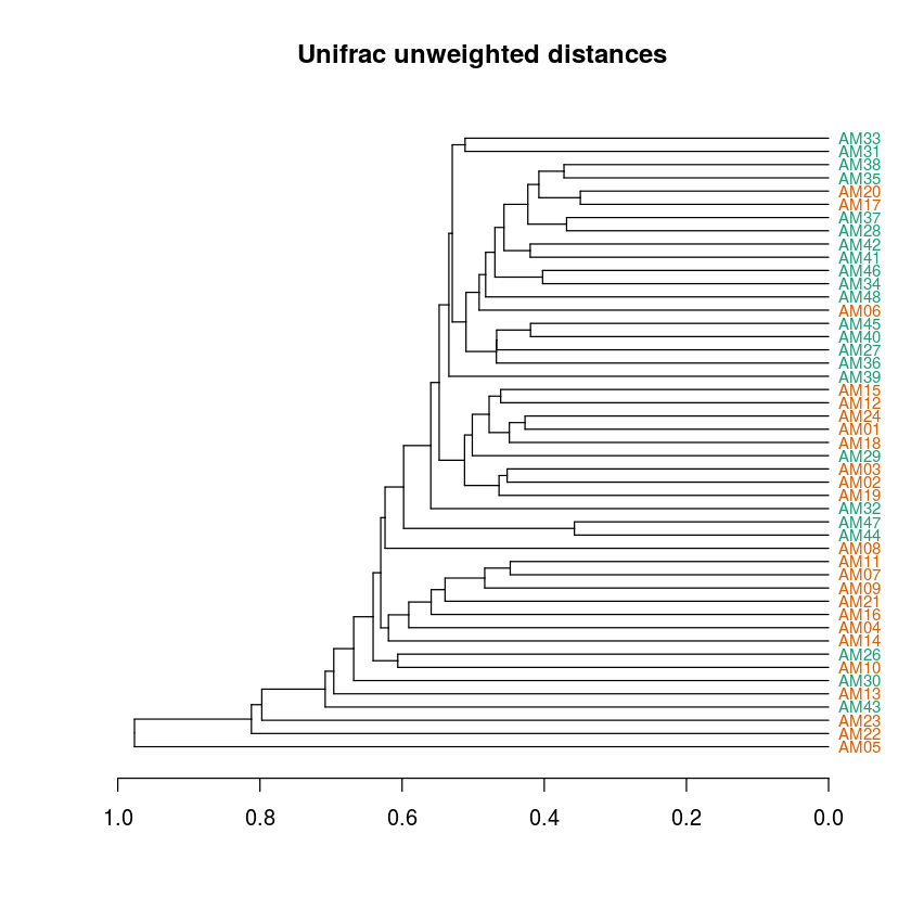
metrito <- get_variable(metro, "sample_type")
sample_data(metro)$metrito <- factor(metrito)
colorCodes <- levels(metrito)
library(doParallel)
library(RColorBrewer)
#sample_data(march_subset)
# camaronUF <- dist(metro, "bray")
camaronUF <- distance(metro, method='bray')
#colorScale <- colors()[c(26,51,76)]
#colorScale <-rainbow(length(levels(get_variable(march_subset, "marchantita"))))
colorScale <- brewer.pal(length(levels(get_variable(metro, "metrito"))),"Dark2")
#colorScale
cols <- colorScale[get_variable(metro, "metrito")]
#cols
#march.tip.labels <- as(get_variable(march_subset, "marchantita"), "character")
# This is the actual hierarchical clustering call, specifying average-link clustering
camaron.hclust <- hclust(camaronUF, method="average")
library(dendextend)
dend <- as.dendrogram(camaron.hclust)
labels_colors(dend) <- cols[order.dendrogram(dend)]
dend %>% set("labels_cex", .75) %>% plot(main="Unifrac unweighted distances",horiz=T)
#ggplot(dend, horiz=T)
phyloseq-class experiment-level object
otu_table()   OTU Table:         [ 22673 taxa and 47 samples ]
sample_data() Sample Data:       [ 47 samples by 29 sample variables ]
tax_table()   Taxonomy Table:    [ 22673 taxa by 6 taxonomic ranks ]


Warning message in brewer.pal(length(levels(get_variable(metro, "metrito"))), "Dark2"):
“minimal value for n is 3, returning requested palette with 3 different levels
”
---------------------
Welcome to dendextend version 1.10.0
Type citation('dendextend') for how to cite the package.

Type browseVignettes(package = 'dendextend') for the package vignette.
The github page is: https://github.com/talgalili/dendextend/

Suggestions and bug-reports can be submitted at: https://github.com/talgalili/dendextend/issues
Or contact: <tal.galili@gmail.com>

	To suppress this message use:  suppressPackageStartupMessages(library(dendextend))
---------------------


Attaching package: ‘dendextend’

The following objects are masked from ‘package:ape’:

    ladderize, rotate

The following object is masked from ‘package:permute’:

    shuffle

The following object is masked from ‘package:stats’:

    cutree
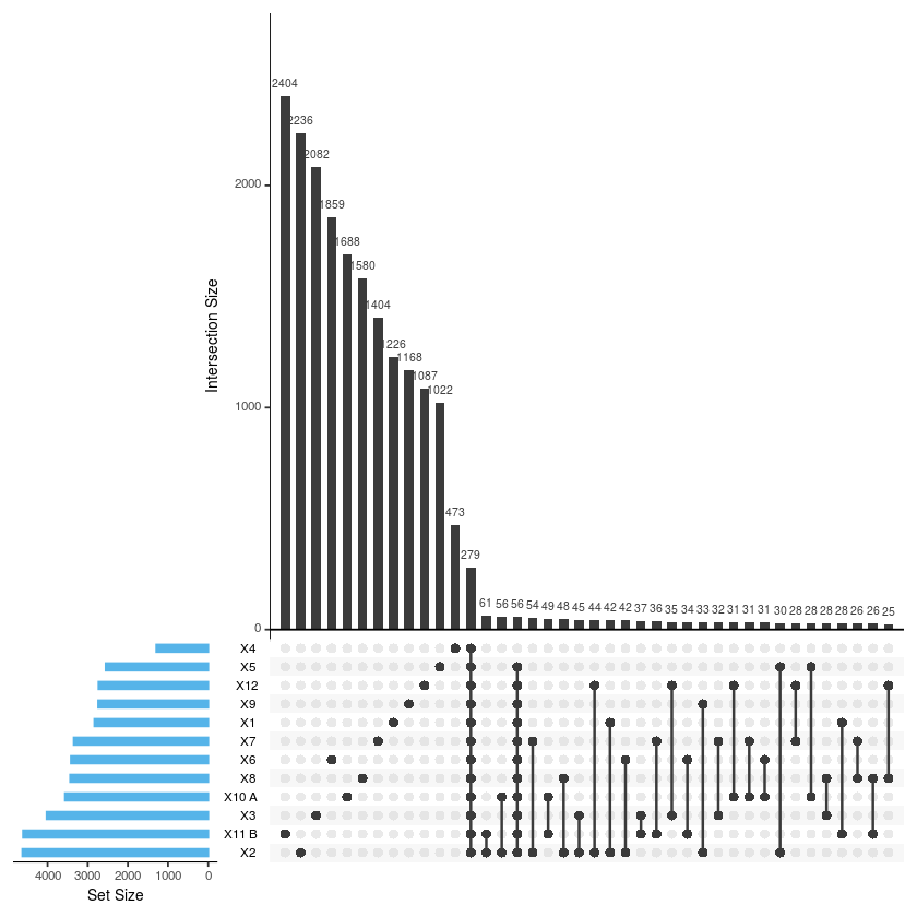
library(UpSetR)
library(grid)
merge2 = merge_samples(metro, "line_number")
merge2 <- as.table(t(otu_table(merge2)))
merge2 <- replace(merge2, merge2>0, 1)
write.table(merge2,"merge2.tmp")

merge2 <- read.table("merge2.tmp", header=TRUE, row.names = 1)
head(merge2)
#merge2[order(rowSums(merge2),decreasing=T),] #
upset(merge2, sets = c('X1','X2','X3','X4','X5','X6','X7','X8','X9','X10.A.','X11.B.', 'X12'),
      sets.bar.color = "#56B4E9", order.by = "freq", empty.intersections = "on")
| <th scope=col>X1</th><th scope=col>X10.A.</th><th scope=col>X11.B.</th><th scope=col>X12</th><th scope=col>X2</th><th scope=col>X3</th><th scope=col>X4</th><th scope=col>X5</th><th scope=col>X6</th><th scope=col>X7</th><th scope=col>X8</th><th scope=col>X9</th> | |||||||||||
|---|---|---|---|---|---|---|---|---|---|---|---|
| 1 | 1 | 1 | 1 | 1 | 1 | 1 | 1 | 1 | 1 | 1 | 1 |
| 1 | 1 | 1 | 1 | 1 | 1 | 1 | 1 | 1 | 1 | 1 | 1 |
| 1 | 1 | 1 | 1 | 1 | 1 | 1 | 1 | 1 | 1 | 1 | 1 |
| 1 | 1 | 1 | 1 | 1 | 1 | 1 | 1 | 1 | 1 | 1 | 1 |
| 1 | 1 | 1 | 1 | 1 | 1 | 1 | 1 | 1 | 1 | 1 | 1 |
| 1 | 1 | 1 | 1 | 1 | 1 | 1 | 1 | 1 | 1 | 1 | 1 |
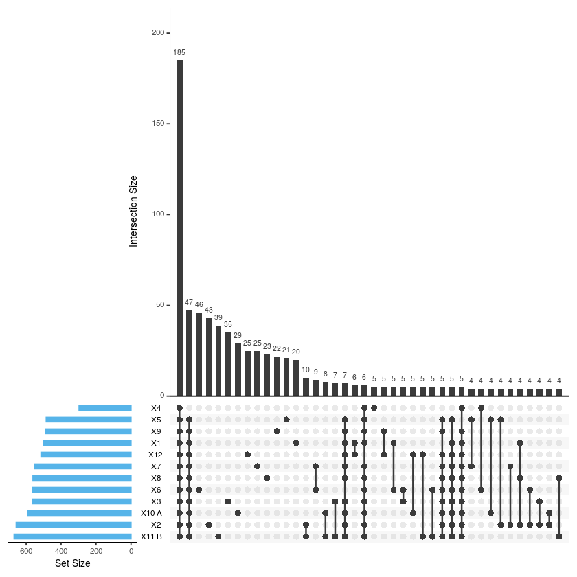
x3 <- tax_glom(metro, taxrank="Genus")
merge2 = merge_samples(x3, "line_number")
merge2 <- as.table(t(otu_table(merge2)))
merge2 <- replace(merge2, merge2>0, 1)
write.table(merge2,"merge2.tmp")

merge2 <- read.table("merge2.tmp", header=TRUE, row.names = 1)
head(merge2)
#merge2[order(rowSums(merge2),decreasing=T),] #
upset(merge2, sets = c('X1','X2','X3','X4','X5','X6','X7','X8','X9','X10.A.','X11.B.', 'X12'),
      sets.bar.color = "#56B4E9", order.by = "freq", empty.intersections = "on")


upset(merge2, sets = c('X1','X2','X3','X4','X5','X6','X7','X8','X9','X10.A.','X11.B.', 'X12'),
      sets.bar.color = "#56B4E9", order.by = "freq", empty.intersections = "on")
ggsave("upset_lines.pdf", width= 10, height= 10, onefile=FALSE)
| <th scope=col>X1</th><th scope=col>X10.A.</th><th scope=col>X11.B.</th><th scope=col>X12</th><th scope=col>X2</th><th scope=col>X3</th><th scope=col>X4</th><th scope=col>X5</th><th scope=col>X6</th><th scope=col>X7</th><th scope=col>X8</th><th scope=col>X9</th> | |||||||||||
|---|---|---|---|---|---|---|---|---|---|---|---|
| 1 | 1 | 1 | 1 | 1 | 1 | 1 | 1 | 1 | 1 | 1 | 1 |
| 1 | 1 | 1 | 1 | 1 | 1 | 1 | 1 | 1 | 1 | 1 | 1 |
| 1 | 1 | 1 | 1 | 1 | 1 | 1 | 1 | 1 | 1 | 1 | 1 |
| 1 | 1 | 1 | 1 | 1 | 1 | 1 | 1 | 1 | 1 | 1 | 1 |
| 1 | 1 | 1 | 1 | 1 | 1 | 1 | 1 | 1 | 1 | 1 | 1 |
| 1 | 1 | 1 | 1 | 1 | 1 | 1 | 1 | 1 | 1 | 1 | 1 |

#Función para calcular las intersecciones get_intersect_members


get_intersect_members <- function (x, ...){
  require(dplyr)
  require(tibble)
  x <- x[,sapply(x, is.numeric)][,0<=colMeans(x[,sapply(x, is.numeric)],na.rm=T) & colMeans(x[,sapply(x, is.numeric)],na.rm=T)<=1]
  n <- names(x)
  x %>% rownames_to_column() -> x
  l <- c(...)
  a <- intersect(names(x), l)
  ar <- vector('list',length(n)+1)
  ar[[1]] <- x
  i=2
  for (item in n) {
    if (item %in% a){
      if (class(x[[item]])=='integer'){
        ar[[i]] <- paste(item, '>= 1')
        i <- i + 1
      }
    } else {
      if (class(x[[item]])=='integer'){
        ar[[i]] <- paste(item, '== 0')
        i <- i + 1
      }
    }
  }
  do.call(filter_, ar) %>% column_to_rownames() -> x
  return(x)
}
intersect <- get_intersect_members(merge2,c('X1','X2','X3','X4','X5','X6','X7','X8','X9','X10.A.','X11.B.', 'X12')) #intersección del core, se puede cambiar para cualquier subconjunto de intersecciones!
length(row.names(intersect)) #número de elementos del core

intersect <- (row.names(intersect)) #identidades del core
vec <- setNames(nm=c(intersect))
# vec
185
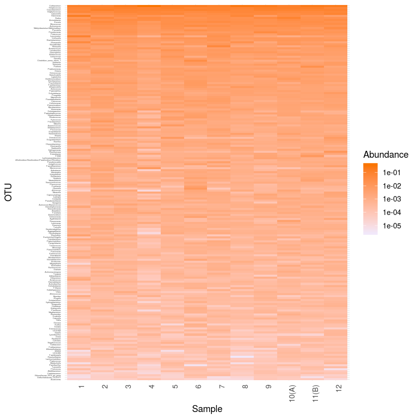
physeqsubsetOTU <- subset_taxa(x3, rownames(tax_table(x3)) %in% vec)
mergeph1 <- merge_samples(physeqsubsetOTU, "line_number")
mergeph1 = transform_sample_counts(mergeph1,function(x) x/sum(x))

    write.table(t(otu_table(mergeph1)),"heatmap_core-lineas.csv",sep="\t")
     write.table(tax_table(mergeph1),"heatmap_core-lineas.tax.csv",sep="\t")
    system("paste heatmap_core-lineas.csv heatmap_core-lineas.tax.csv >heatmap_core-lineas.otutax.csv" )

t1 <- as.data.frame(colSums(otu_table(mergeph1)))

# write.table(t, "vennupset.txt")
t <-(tax_table(mergeph1)) #hago esto porque el melt sobre este objeto phyloseq no trabaja, creo que hay que usar psmelt para esto

write.table(t, "taxvennupset.txt")
t <- as.data.frame(read.table("taxvennupset.txt", header=T, row.names = 1))

# system("paste vennupset.txt taxvennupset.txt >coreupset.txt")

# read.table("coreupset.txt", header=T, sep="\t")
t3 <- merge(t,t1, by=0, all=TRUE )

    head(t3)
names(t3)[8] <-"abundance"

t4 <- t3[order(-t3$abundance),]
write.table(t4, "taxvennupset-Entrada-Salida.txt")
 t5 <-   as.vector(t4$Row.names)
t5
t4
summary(t4)


p <- plot_bar(mergeph1, "Genus")

yx <- p$data

    yx <- as.data.frame(yx)
head(yx)
yx <- yx[order(-yx$Abundance),]

head(yx)
levels1=c('1','2','3','4','5','6','7','8','9','10(A)','11(B)','12')
levels1
levels2 = rev(t5)

yx$orden <- factor(yx$Sample, levels = levels1)
yx$abun <- factor(yx$OTU, levels= levels2)
head(yx$abun)

                                     #Correción a valores vacios en Género

    ylabvec = as(tax_table(mergeph1)[,"Genus"], "character")
names(ylabvec) <- taxa_names(mergeph1)
ylabvec[is.na(ylabvec)] <- ""

    #####

# ggplot(data=yx, aes(x = yx$orden, y= reorder(Genus, Abundance), fill= Abundance))  +
#    geom_raster() + theme_minimal () +
#    xlab("") + ylab("") +
#    scale_fill_gradient(low="#bebebe", high="#000000", na.value = "white", trans = "log10") +
#    theme(axis.text.x = element_text( angle = 90, hjust = 1),
#          axis.text.y = element_text(size = 4.2))
| ASV_1 | Bacteria | Actinobacteriota | Actinobacteria | Propionibacteriales | Propionibacteriaceae | Cutibacterium | 2.290667670 |
| ASV_1007 | Bacteria | Firmicutes | Clostridia | Clostridia_or | Hungateiclostridiaceae | Fastidiosipila | 0.001820265 |
| ASV_101 | Bacteria | Proteobacteria | Alphaproteobacteria | Azospirillales | Azospirillaceae | Skermanella | 0.020332544 |
| ASV_1027 | Bacteria | Firmicutes | Clostridia | Peptostreptococcales-Tissierellales | Peptostreptococcales-Tissierellales_fa | Murdochiella | 0.001554152 |
| ASV_1039 | Bacteria | Bacteroidota | Bacteroidia | Cytophagales | Hymenobacteraceae | Adhaeribacter | 0.005039240 |
| ASV_1044 | Bacteria | Firmicutes | Clostridia | Lachnospirales | Lachnospiraceae | Lachnoclostridium | 0.001689947 |
<ol class=list-inline> <li>‘ASV_1’</li> <li>‘ASV_2’</li> <li>‘ASV_6’</li> <li>‘ASV_5’</li> <li>‘ASV_4’</li> <li>‘ASV_3’</li> <li>‘ASV_13’</li> <li>‘ASV_26’</li> <li>‘ASV_19’</li> <li>‘ASV_9’</li> <li>‘ASV_70’</li> <li>‘ASV_18’</li> <li>‘ASV_90’</li> <li>‘ASV_96’</li> <li>‘ASV_17’</li> <li>‘ASV_16’</li> <li>‘ASV_43’</li> <li>‘ASV_28’</li> <li>‘ASV_14’</li> <li>‘ASV_304’</li> <li>‘ASV_31’</li> <li>‘ASV_58’</li> <li>‘ASV_129’</li> <li>‘ASV_42’</li> <li>‘ASV_35’</li> <li>‘ASV_27’</li> <li>‘ASV_41’</li> <li>‘ASV_123’</li> <li>‘ASV_32’</li> <li>‘ASV_82’</li> <li>‘ASV_91’</li> <li>‘ASV_251’</li> <li>‘ASV_66’</li> <li>‘ASV_56’</li> <li>‘ASV_62’</li> <li>‘ASV_184’</li> <li>‘ASV_171’</li> <li>‘ASV_168’</li> <li>‘ASV_95’</li> <li>‘ASV_128’</li> <li>‘ASV_109’</li> <li>‘ASV_36’</li> <li>‘ASV_134’</li> <li>‘ASV_46’</li> <li>‘ASV_52’</li> <li>‘ASV_206’</li> <li>‘ASV_60’</li> <li>‘ASV_54’</li> <li>‘ASV_270’</li> <li>‘ASV_265’</li> <li>‘ASV_412’</li> <li>‘ASV_106’</li> <li>‘ASV_68’</li> <li>‘ASV_77’</li> <li>‘ASV_97’</li> <li>‘ASV_202’</li> <li>‘ASV_137’</li> <li>‘ASV_455’</li> <li>‘ASV_256’</li> <li>‘ASV_74’</li> <li>‘ASV_317’</li> <li>‘ASV_67’</li> <li>‘ASV_117’</li> <li>‘ASV_126’</li> <li>‘ASV_150’</li> <li>‘ASV_118’</li> <li>‘ASV_110’</li> <li>‘ASV_471’</li> <li>‘ASV_253’</li> <li>‘ASV_101’</li> <li>‘ASV_238’</li> <li>‘ASV_447’</li> <li>‘ASV_360’</li> <li>‘ASV_259’</li> <li>‘ASV_125’</li> <li>‘ASV_193’</li> <li>‘ASV_541’</li> <li>‘ASV_397’</li> <li>‘ASV_170’</li> <li>‘ASV_245’</li> <li>‘ASV_138’</li> <li>‘ASV_450’</li> <li>‘ASV_112’</li> <li>‘ASV_136’</li> <li>‘ASV_151’</li> <li>‘ASV_342’</li> <li>‘ASV_274’</li> <li>‘ASV_194’</li> <li>‘ASV_485’</li> <li>‘ASV_431’</li> <li>‘ASV_469’</li> <li>‘ASV_220’</li> <li>‘ASV_543’</li> <li>‘ASV_367’</li> <li>‘ASV_178’</li> <li>‘ASV_1064’</li> <li>‘ASV_215’</li> <li>‘ASV_681’</li> <li>‘ASV_153’</li> <li>‘ASV_510’</li> <li>‘ASV_320’</li> <li>‘ASV_285’</li> <li>‘ASV_191’</li> <li>‘ASV_433’</li> <li>‘ASV_651’</li> <li>‘ASV_214’</li> <li>‘ASV_372’</li> <li>‘ASV_250’</li> <li>‘ASV_174’</li> <li>‘ASV_388’</li> <li>‘ASV_482’</li> <li>‘ASV_357’</li> <li>‘ASV_2015’</li> <li>‘ASV_188’</li> <li>‘ASV_204’</li> <li>‘ASV_226’</li> <li>‘ASV_219’</li> <li>‘ASV_849’</li> <li>‘ASV_319’</li> <li>‘ASV_519’</li> <li>‘ASV_355’</li> <li>‘ASV_440’</li> <li>‘ASV_407’</li> <li>‘ASV_449’</li> <li>‘ASV_901’</li> <li>‘ASV_435’</li> <li>‘ASV_386’</li> <li>‘ASV_553’</li> <li>‘ASV_418’</li> <li>‘ASV_815’</li> <li>‘ASV_873’</li> <li>‘ASV_1379’</li> <li>‘ASV_1110’</li> <li>‘ASV_1039’</li> <li>‘ASV_445’</li> <li>‘ASV_678’</li> <li>‘ASV_326’</li> <li>‘ASV_942’</li> <li>‘ASV_3196’</li> <li>‘ASV_375’</li> <li>‘ASV_609’</li> <li>‘ASV_830’</li> <li>‘ASV_590’</li> <li>‘ASV_999’</li> <li>‘ASV_755’</li> <li>‘ASV_684’</li> <li>‘ASV_2142’</li> <li>‘ASV_963’</li> <li>‘ASV_1060’</li> <li>‘ASV_480’</li> <li>‘ASV_1254’</li> <li>‘ASV_525’</li> <li>‘ASV_1623’</li> <li>‘ASV_659’</li> <li>‘ASV_836’</li> <li>‘ASV_2541’</li> <li>‘ASV_1137’</li> <li>‘ASV_935’</li> <li>‘ASV_1869’</li> <li>‘ASV_518’</li> <li>‘ASV_1186’</li> <li>‘ASV_3882’</li> <li>‘ASV_1472’</li> <li>‘ASV_931’</li> <li>‘ASV_2005’</li> <li>‘ASV_1719’</li> <li>‘ASV_1342’</li> <li>‘ASV_2962’</li> <li>‘ASV_1965’</li> <li>‘ASV_1348’</li> <li>‘ASV_1752’</li> <li>‘ASV_2924’</li> <li>‘ASV_1007’</li> <li>‘ASV_3880’</li> <li>‘ASV_1044’</li> <li>‘ASV_1984’</li> <li>‘ASV_1027’</li> <li>‘ASV_4864’</li> <li>‘ASV_1196’</li> <li>‘ASV_2195’</li> <li>‘ASV_5031’</li> <li>‘ASV_1440’</li> <li>‘ASV_4584’</li> <li>‘ASV_3549’</li> <li>‘ASV_1973’</li> </ol>
| <th scope=col>Row.names</th><th scope=col>Kingdom</th><th scope=col>Phylum</th><th scope=col>Class</th><th scope=col>Order</th><th scope=col>Family</th><th scope=col>Genus</th><th scope=col>abundance</th> | |||||||
|---|---|---|---|---|---|---|---|
| ASV_1 | Bacteria | Actinobacteriota | Actinobacteria | Propionibacteriales | Propionibacteriaceae | Cutibacterium | 2.29066767 |
| ASV_2 | Bacteria | Firmicutes | Bacilli | Lactobacillales | Streptococcaceae | Streptococcus | 1.11725948 |
| ASV_6 | Bacteria | Actinobacteriota | Actinobacteria | Corynebacteriales | Corynebacteriaceae | Corynebacterium | 1.06249797 |
| ASV_5 | Bacteria | Firmicutes | Bacilli | Staphylococcales | Staphylococcaceae | Staphylococcus | 0.68366594 |
| ASV_4 | Bacteria | Actinobacteriota | Actinobacteria | Corynebacteriales | Corynebacteriaceae | Lawsonella | 0.53559802 |
| ASV_3 | Bacteria | Proteobacteria | Gammaproteobacteria | Oceanospirillales | Halomonadaceae | Halomonas | 0.40929609 |
| ASV_13 | Bacteria | Actinobacteriota | Actinobacteria | Micrococcales | Micrococcaceae | Rothia | 0.39471905 |
| ASV_26 | Bacteria | Proteobacteria | Gammaproteobacteria | Pseudomonadales | Moraxellaceae | Acinetobacter | 0.34119212 |
| ASV_19 | Bacteria | Actinobacteriota | Actinobacteria | Micrococcales | Micrococcaceae | Kocuria | 0.33427959 |
| ASV_9 | Bacteria | Actinobacteriota | Actinobacteria | Micrococcales | Micrococcaceae | Micrococcus | 0.26203884 |
| ASV_70 | Bacteria | Actinobacteriota | Actinobacteria | Actinomycetales | Actinomycetaceae | Actinomyces | 0.25964354 |
| ASV_18 | Bacteria | Proteobacteria | Alphaproteobacteria | Rhizobiales | Beijerinckiaceae | Methylobacterium-Methylorubrum | 0.18500243 |
| ASV_90 | Bacteria | Bacteroidota | Bacteroidia | Bacteroidales | Prevotellaceae | Prevotella | 0.17138229 |
| ASV_96 | Bacteria | Proteobacteria | Gammaproteobacteria | Pseudomonadales | Pseudomonadaceae | Pseudomonas | 0.17136659 |
| ASV_17 | Bacteria | Proteobacteria | Alphaproteobacteria | Rhodobacterales | Rhodobacteraceae | Paracoccus | 0.14373532 |
| ASV_16 | Bacteria | Firmicutes | Bacilli | Lactobacillales | Leuconostocaceae | Leuconostoc | 0.13999839 |
| ASV_43 | Bacteria | Firmicutes | Negativicutes | Veillonellales-Selenomonadales | Veillonellaceae | Veillonella | 0.12991747 |
| ASV_28 | Bacteria | Actinobacteriota | Actinobacteria | Micrococcales | Dermabacteraceae | Brachybacterium | 0.12977183 |
| ASV_14 | Bacteria | Proteobacteria | Gammaproteobacteria | Alteromonadales | Shewanellaceae | Shewanella | 0.12430211 |
| ASV_304 | Bacteria | Actinobacteriota | Actinobacteria | Propionibacteriales | Nocardioidaceae | Nocardioides | 0.09656966 |
| ASV_31 | Bacteria | Firmicutes | Bacilli | Lactobacillales | Leuconostocaceae | Weissella | 0.09483407 |
| ASV_58 | Bacteria | Firmicutes | Clostridia | Peptostreptococcales-Tissierellales | Peptostreptococcales-Tissierellales_fa | Anaerococcus | 0.08978460 |
| ASV_129 | Bacteria | Firmicutes | Bacilli | Lactobacillales | Lactobacillaceae | Lactobacillus | 0.08136070 |
| ASV_42 | Bacteria | Proteobacteria | Gammaproteobacteria | Pasteurellales | Pasteurellaceae | Haemophilus | 0.08001474 |
| ASV_35 | Bacteria | Actinobacteriota | Actinobacteria | Frankiales | Geodermatophilaceae | Blastococcus | 0.07522387 |
| ASV_27 | Bacteria | Firmicutes | Bacilli | Lactobacillales | Streptococcaceae | Lactococcus | 0.07123338 |
| ASV_41 | Bacteria | Firmicutes | Bacilli | Staphylococcales | Gemellaceae | Gemella | 0.06659775 |
| ASV_123 | Bacteria | Firmicutes | Clostridia | Clostridiales | Clostridiaceae | Clostridium_sensu_stricto_1 | 0.06305577 |
| ASV_32 | Bacteria | Actinobacteriota | Actinobacteria | Micrococcales | Intrasporangiaceae | Janibacter | 0.06215911 |
| ASV_82 | Bacteria | Proteobacteria | Gammaproteobacteria | Burkholderiales | Neisseriaceae | Neisseria | 0.06157533 |
| ⋮ | ⋮ | ⋮ | ⋮ | ⋮ | ⋮ | ⋮ | ⋮ |
| ASV_2541 | Bacteria | Patescibacteria | Saccharimonadia | Saccharimonadales | Saccharimonadaceae | TM7a | 0.0033428207 |
| ASV_1137 | Bacteria | Proteobacteria | Alphaproteobacteria | Rhizobiales | Devosiaceae | Devosia | 0.0031977325 |
| ASV_935 | Bacteria | Firmicutes | Bacilli | Bacillales | Planococcaceae | Kurthia | 0.0031532184 |
| ASV_1869 | Bacteria | Proteobacteria | Gammaproteobacteria | Enterobacterales | Yersiniaceae | Serratia | 0.0031374181 |
| ASV_518 | Bacteria | Firmicutes | Bacilli | Lactobacillales | Aerococcaceae | Eremococcus | 0.0027469601 |
| ASV_1186 | Bacteria | Firmicutes | Clostridia | Oscillospirales | Oscillospiraceae | UCG-002 | 0.0026775756 |
| ASV_3882 | Bacteria | Actinobacteriota | Thermoleophilia | Gaiellales | Gaiellaceae | Gaiella | 0.0025280925 |
| ASV_1472 | Bacteria | Firmicutes | Bacilli | Bacillales | Planococcaceae | Lysinibacillus | 0.0025058386 |
| ASV_931 | Bacteria | Firmicutes | Clostridia | Lachnospirales | Lachnospiraceae | Dorea | 0.0025054089 |
| ASV_2005 | Bacteria | Acidobacteriota | Acidobacteriae | Bryobacterales | Bryobacteraceae | Bryobacter | 0.0024479238 |
| ASV_1719 | Bacteria | Proteobacteria | Gammaproteobacteria | Cellvibrionales | Cellvibrionaceae | Cellvibrio | 0.0024149934 |
| ASV_1342 | Bacteria | Firmicutes | Negativicutes | Veillonellales-Selenomonadales | Veillonellaceae | Negativicoccus | 0.0023887852 |
| ASV_2962 | Bacteria | Actinobacteriota | Actinobacteria | Actinomycetales | Actinomycetaceae | Varibaculum | 0.0023235953 |
| ASV_1965 | Bacteria | Synergistota | Synergistia | Synergistales | Synergistaceae | Fretibacterium | 0.0023030874 |
| ASV_1348 | Bacteria | Proteobacteria | Alphaproteobacteria | Sphingomonadales | Sphingomonadaceae | Altererythrobacter | 0.0019679164 |
| ASV_1752 | Bacteria | Firmicutes | Clostridia | Peptostreptococcales-Tissierellales | Peptostreptococcales-Tissierellales_fa | W5053 | 0.0019378517 |
| ASV_2924 | Bacteria | Firmicutes | Clostridia | Oscillospirales | Oscillospiraceae | UCG-005 | 0.0019250371 |
| ASV_1007 | Bacteria | Firmicutes | Clostridia | Clostridia_or | Hungateiclostridiaceae | Fastidiosipila | 0.0018202651 |
| ASV_3880 | Bacteria | Gemmatimonadota | Gemmatimonadetes | Gemmatimonadales | Gemmatimonadaceae | Roseisolibacter | 0.0017879066 |
| ASV_1044 | Bacteria | Firmicutes | Clostridia | Lachnospirales | Lachnospiraceae | Lachnoclostridium | 0.0016899467 |
| ASV_1984 | Bacteria | Firmicutes | Clostridia | Peptococcales | Peptococcaceae | Peptococcus | 0.0016149387 |
| ASV_1027 | Bacteria | Firmicutes | Clostridia | Peptostreptococcales-Tissierellales | Peptostreptococcales-Tissierellales_fa | Murdochiella | 0.0015541522 |
| ASV_4864 | Bacteria | Firmicutes | Bacilli | Paenibacillales | Paenibacillaceae | Paenibacillus | 0.0015324177 |
| ASV_1196 | Bacteria | Bacteroidota | Bacteroidia | Bacteroidales | Tannerellaceae | Tannerella | 0.0014439009 |
| ASV_2195 | Bacteria | Firmicutes | Bacilli | Lactobacillales | Streptococcaceae | Floricoccus | 0.0013014153 |
| ASV_5031 | Bacteria | Abditibacteriota | Abditibacteria | Abditibacteriales | Abditibacteriaceae | Abditibacterium | 0.0011572429 |
| ASV_1440 | Bacteria | Proteobacteria | Gammaproteobacteria | Cardiobacteriales | Cardiobacteriaceae | Cardiobacterium | 0.0011498768 |
| ASV_4584 | Bacteria | Bacteroidota | Bacteroidia | Bacteroidales | Rikenellaceae | Rikenellaceae_RC9_gut_group | 0.0011047558 |
| ASV_3549 | Bacteria | Firmicutes | Clostridia | Lachnospirales | Defluviitaleaceae | Defluviitaleaceae_UCG-011 | 0.0005573410 |
| ASV_1973 | Bacteria | Actinobacteriota | Actinobacteria | Micrococcales | Micrococcaceae | Acaricomes | 0.0005485926 |
  Row.names             Kingdom                 Phylum
 Length:185         Bacteria:185   Firmicutes      :70
 Class :AsIs                       Actinobacteriota:50
 Mode  :character                  Proteobacteria  :40
                                   Bacteroidota    :15
                                   Deinococcota    : 2
                                   Fusobacteriota  : 2
                                   (Other)         : 6
                 Class                                    Order
 Actinobacteria     :46   Micrococcales                      : 24
 Bacilli            :33   Lactobacillales                    : 18
 Clostridia         :31   Peptostreptococcales-Tissierellales: 14
 Gammaproteobacteria:28   Lachnospirales                     :  9
 Bacteroidia        :15   Corynebacteriales                  :  7
 Alphaproteobacteria:12   Staphylococcales                   :  7
 (Other)            :20   (Other)                            :106
                                    Family                Genus
 Micrococcaceae                        :  9   Abditibacterium:  1
 Lachnospiraceae                       :  8   Abiotrophia    :  1
 Peptostreptococcales-Tissierellales_fa:  8   Acaricomes     :  1
 Carnobacteriaceae                     :  6   Acidovorax     :  1
 Staphylococcaceae                     :  6   Acinetobacter  :  1
 Peptostreptococcaceae                 :  5   Actinobacillus :  1
 (Other)                               :143   (Other)        :179
   abundance
 Min.   :0.0005486
 1st Qu.:0.0045952
 Median :0.0131576
 Mean   :0.0648649
 3rd Qu.:0.0379244
 Max.   :2.2906677
| <th scope=col>OTU</th><th scope=col>Sample</th><th scope=col>Abundance</th><th scope=col>id</th><th scope=col>sample_location</th><th scope=col>sample_id</th><th scope=col>line_number</th><th scope=col>sample_type</th><th scope=col>date</th><th scope=col>time</th><th scope=col>⋯</th><th scope=col>Chao1</th><th scope=col>Shannon</th><th scope=col>Simpson</th><th scope=col>metrito</th><th scope=col>Kingdom</th><th scope=col>Phylum</th><th scope=col>Class</th><th scope=col>Order</th><th scope=col>Family</th><th scope=col>Genus</th> | ||||||||||||||||||||
|---|---|---|---|---|---|---|---|---|---|---|---|---|---|---|---|---|---|---|---|---|
| ASV_1 | 4 | 0.3753143 | 30.5 | 23.00000 | 33.00000 | 7 | 1.000000 | 1.0 | 21.00000 | ⋯ | 14102.46 | 6.122639 | 0.9801934 | 1.000000 | Bacteria | Actinobacteriota | Actinobacteria | Propionibacteriales | Propionibacteriaceae | Cutibacterium |
| ASV_1 | 8 | 0.2685063 | 25.0 | 17.25000 | 26.50000 | 11 | 1.500000 | 2.5 | 17.75000 | ⋯ | 18272.34 | 6.422750 | 0.9801182 | 1.500000 | Bacteria | Actinobacteriota | Actinobacteria | Propionibacteriales | Propionibacteriaceae | Cutibacterium |
| ASV_1 | 11(B) | 0.2211542 | 21.8 | 13.20000 | 25.00000 | 3 | 1.600000 | 1.6 | 17.60000 | ⋯ | 17894.83 | 6.613091 | 0.9839803 | 1.600000 | Bacteria | Actinobacteriota | Actinobacteria | Propionibacteriales | Propionibacteriaceae | Cutibacterium |
| ASV_1 | 9 | 0.2142901 | 26.0 | 17.25000 | 26.25000 | 12 | 1.500000 | 4.5 | 30.75000 | ⋯ | 12867.00 | 6.131456 | 0.9873997 | 1.500000 | Bacteria | Actinobacteriota | Actinobacteria | Propionibacteriales | Propionibacteriaceae | Cutibacterium |
| ASV_1 | 3 | 0.2041766 | 23.6 | 17.00000 | 18.00000 | 6 | 1.600000 | 2.2 | 19.20000 | ⋯ | 18923.90 | 6.901101 | 0.9882069 | 1.600000 | Bacteria | Actinobacteriota | Actinobacteria | Propionibacteriales | Propionibacteriaceae | Cutibacterium |
| ASV_1 | 12 | 0.1933069 | 23.0 | 22.66667 | 30.66667 | 4 | 1.333333 | 6.0 | 17.33333 | ⋯ | 12046.64 | 6.021041 | 0.9830369 | 1.333333 | Bacteria | Actinobacteriota | Actinobacteria | Propionibacteriales | Propionibacteriaceae | Cutibacterium |
<ol class=list-inline> <li>‘1’</li> <li>‘2’</li> <li>‘3’</li> <li>‘4’</li> <li>‘5’</li> <li>‘6’</li> <li>‘7’</li> <li>‘8’</li> <li>‘9’</li> <li>‘10(A)’</li> <li>‘11(B)’</li> <li>‘12’</li> </ol>
<ol class=list-inline> <li>ASV_1</li> <li>ASV_1</li> <li>ASV_1</li> <li>ASV_1</li> <li>ASV_1</li> <li>ASV_1</li> </ol>
Scale for 'fill' is already present. Adding another scale for 'fill', which
will replace the existing scale.

plot_heatmap(mergeph1, "NULL", sample.order=levels1, taxa.order=rev(t5)) + scale_y_discrete(labels=ylabvec)  + theme_minimal () +
   scale_fill_gradient(low="#F1E8FA", high="#FA7500", na.value = "white", trans = "log10")  +
   theme(axis.text.x = element_text( angle = 90, hjust = 1),
         axis.text.y = element_text(size = 2.5))

 ggsave ("heatmap_core.pdf", width=20, height=80, units="cm")
Scale for 'fill' is already present. Adding another scale for 'fill', which
will replace the existing scale.
library(DESeq2)
library(RColorBrewer)
library(ggplot2)
library(phyloseq)
library(plyr)

metro_sig=subset_samples(metro, sample_type !="NA" )
metro_sig
obj1deseq = phyloseq_to_deseq2(metro_sig, ~sample_type)


gm_mean = function(x, na.rm=TRUE){
  exp(sum(log(x[x > 0]), na.rm=na.rm) / length(x))
}

geoMeans = apply(counts(obj1deseq), 1, gm_mean)
obj1deseq = estimateSizeFactors(obj1deseq, geoMeans = geoMeans)

##adición de la viñeta para el error de la media de 0s
obj1deseq = DESeq(obj1deseq, fitType="local")

#obj1deseq = DESeq(obj1deseq, test="Wald", fitType="parametric")
Loading required package: S4Vectors
Loading required package: stats4
Loading required package: BiocGenerics

Attaching package: ‘BiocGenerics’

The following objects are masked from ‘package:parallel’:

    clusterApply, clusterApplyLB, clusterCall, clusterEvalQ,
    clusterExport, clusterMap, parApply, parCapply, parLapply,
    parLapplyLB, parRapply, parSapply, parSapplyLB

The following objects are masked from ‘package:dplyr’:

    combine, intersect, setdiff, union

The following objects are masked from ‘package:stats’:

    IQR, mad, sd, var, xtabs

The following objects are masked from ‘package:base’:

    anyDuplicated, append, as.data.frame, basename, cbind, colMeans,
    colnames, colSums, dirname, do.call, duplicated, eval, evalq,
    Filter, Find, get, grep, grepl, intersect, is.unsorted, lapply,
    lengths, Map, mapply, match, mget, order, paste, pmax, pmax.int,
    pmin, pmin.int, Position, rank, rbind, Reduce, rowMeans, rownames,
    rowSums, sapply, setdiff, sort, table, tapply, union, unique,
    unsplit, which, which.max, which.min


Attaching package: ‘S4Vectors’

The following objects are masked from ‘package:dplyr’:

    first, rename

The following object is masked from ‘package:tidyr’:

    expand

The following object is masked from ‘package:base’:

    expand.grid

Loading required package: IRanges

Attaching package: ‘IRanges’

The following object is masked from ‘package:phyloseq’:

    distance

The following objects are masked from ‘package:dplyr’:

    collapse, desc, slice

The following object is masked from ‘package:purrr’:

    reduce

Loading required package: GenomicRanges
Loading required package: GenomeInfoDb
Loading required package: SummarizedExperiment
Loading required package: Biobase
Welcome to Bioconductor

    Vignettes contain introductory material; view with
    'browseVignettes()'. To cite Bioconductor, see
    'citation("Biobase")', and for packages 'citation("pkgname")'.


Attaching package: ‘Biobase’

The following object is masked from ‘package:phyloseq’:

    sampleNames

Loading required package: DelayedArray
Loading required package: matrixStats

Attaching package: ‘matrixStats’

The following objects are masked from ‘package:Biobase’:

    anyMissing, rowMedians

The following object is masked from ‘package:dplyr’:

    count

Loading required package: BiocParallel

Attaching package: ‘DelayedArray’

The following objects are masked from ‘package:matrixStats’:

    colMaxs, colMins, colRanges, rowMaxs, rowMins, rowRanges

The following object is masked from ‘package:purrr’:

    simplify

The following objects are masked from ‘package:base’:

    aperm, apply

------------------------------------------------------------------------------
You have loaded plyr after dplyr - this is likely to cause problems.
If you need functions from both plyr and dplyr, please load plyr first, then dplyr:
library(plyr); library(dplyr)
------------------------------------------------------------------------------

Attaching package: ‘plyr’

The following object is masked from ‘package:matrixStats’:

    count

The following object is masked from ‘package:IRanges’:

    desc

The following object is masked from ‘package:S4Vectors’:

    rename

The following objects are masked from ‘package:dplyr’:

    arrange, count, desc, failwith, id, mutate, rename, summarise,
    summarize

The following object is masked from ‘package:purrr’:

    compact


phyloseq-class experiment-level object
otu_table()   OTU Table:         [ 22673 taxa and 47 samples ]
sample_data() Sample Data:       [ 47 samples by 29 sample variables ]
tax_table()   Taxonomy Table:    [ 22673 taxa by 6 taxonomic ranks ]


converting counts to integer mode
using pre-existing size factors
estimating dispersions
gene-wise dispersion estimates
mean-dispersion relationship
final dispersion estimates
fitting model and testing
-- replacing outliers and refitting for 8421 genes
-- DESeq argument 'minReplicatesForReplace' = 7
-- original counts are preserved in counts(dds)
estimating dispersions
fitting model and testing
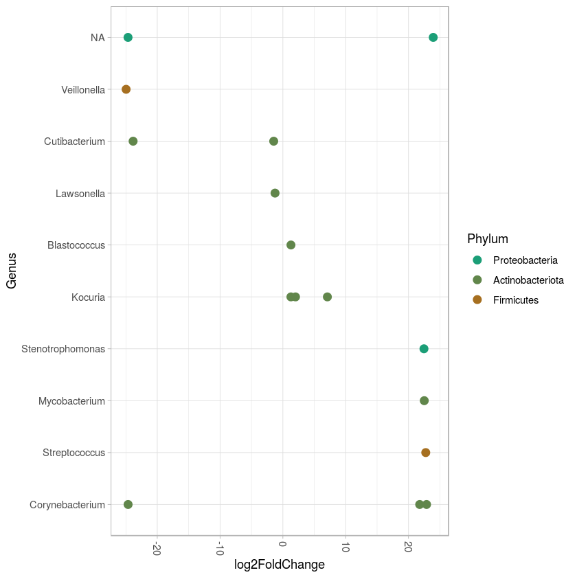
res = results(obj1deseq, cooksCutoff = FALSE)
# quick explanation of Cook's distance: it measures within each gene, for each sample, how removing that sample would change the LFCs (all of the coefficients implied by the design and estimated by DESeq2). So if you have e.g. 3 samples vs 2 samples, and the counts for a gene are [10,10,10] vs [15, 1000], you can see how the Cook's distance will be high for the two samples. Removing either one changes the LFC for the comparison of the two groups. However, if it were [10,10,10] vs [50,50], the two samples "support" each other, such that removing one doesn't change the LFC at all. Hence, we find Cook's to be useful for identifying outliers.
alpha = 0.01
sigtab = res[which(res$padj < alpha), ]
sigtab = cbind(as(sigtab, "data.frame"), as(tax_table(metro_sig)[rownames(sigtab), ], "matrix"))
# Phylum order
x = tapply(sigtab$log2FoldChange, sigtab$Phylum, function(x) max(x))
x = sort(x, TRUE)
sigtab$Phylum = factor(as.character(sigtab$Phylum), levels=names(x))
# Genus order
x = tapply(sigtab$log2FoldChange, sigtab$Genus, function(x) max(x))
x = sort(x, TRUE)
sigtab$Genus = factor(as.character(sigtab$Genus), levels=names(x))

ggplot(sigtab, aes(x=Genus, y=log2FoldChange, color=Phylum)) + scale_color_manual(values=colorRampPalette(brewer.pal(8,"Dark2"))(20))+geom_point(size=3)+theme_light() +theme(axis.text.x = element_text(angle = -90, hjust = 0, vjust=0.5)) + coord_flip()
#sigtab
#ggsave ("torniquete_pasamanos_SIG.pdf", width=30, height=15, units="cm")
sigtab

 write.table(sigtab,"handrail-turnstileOR.csv",sep="\t")
| <th scope=col>baseMean</th><th scope=col>log2FoldChange</th><th scope=col>lfcSE</th><th scope=col>stat</th><th scope=col>pvalue</th><th scope=col>padj</th><th scope=col>Kingdom</th><th scope=col>Phylum</th><th scope=col>Class</th><th scope=col>Order</th><th scope=col>Family</th><th scope=col>Genus</th> | |||||||||||
|---|---|---|---|---|---|---|---|---|---|---|---|
| 16132.859322 | -1.459546 | 0.3683595 | -3.962286 | 7.423561e-05 | 6.475629e-03 | Bacteria | Actinobacteriota | Actinobacteria | Propionibacteriales | Propionibacteriaceae | Cutibacterium |
| 2146.727806 | -1.246392 | 0.3191419 | -3.905448 | 9.405103e-05 | 7.110258e-03 | Bacteria | Actinobacteriota | Actinobacteria | Corynebacteriales | Corynebacteriaceae | Lawsonella |
| 497.860423 | 2.009594 | 0.4142819 | 4.850790 | 1.229709e-06 | 1.267718e-04 | Bacteria | Actinobacteriota | Actinobacteria | Micrococcales | Micrococcaceae | Kocuria |
| 469.021045 | 1.278936 | 0.3325598 | 3.845732 | 1.201930e-04 | 8.518676e-03 | Bacteria | Actinobacteriota | Actinobacteria | Micrococcales | Micrococcaceae | Kocuria |
| 286.296527 | 1.286759 | 0.3289152 | 3.912130 | 9.148558e-05 | 7.110258e-03 | Bacteria | Actinobacteriota | Actinobacteria | Frankiales | Geodermatophilaceae | Blastococcus |
| 12.696749 | -24.642029 | 2.9166383 | -8.448778 | 2.943678e-17 | 5.563552e-15 | Bacteria | Actinobacteriota | Actinobacteria | Corynebacteriales | Corynebacteriaceae | Corynebacterium |
| 22.251272 | 23.939615 | 2.0813607 | 11.501906 | 1.290340e-30 | 1.463246e-27 | Bacteria | Proteobacteria | Alphaproteobacteria | Rickettsiales | Mitochondria | NA |
| 7.071797 | -23.844134 | 2.9172184 | -8.173586 | 2.993568e-16 | 4.849580e-14 | Bacteria | Actinobacteriota | Actinobacteria | Propionibacteriales | Propionibacteriaceae | Cutibacterium |
| 10.375836 | 22.875134 | 2.9179937 | 7.839336 | 4.529343e-15 | 6.420344e-13 | Bacteria | Actinobacteriota | Actinobacteria | Corynebacteriales | Corynebacteriaceae | Corynebacterium |
| 16.617408 | 21.782770 | 2.9176957 | 7.465744 | 8.283011e-14 | 9.392935e-12 | Bacteria | Actinobacteriota | Actinobacteria | Corynebacteriales | Corynebacteriaceae | Corynebacterium |
| 7.981757 | 22.510169 | 2.4877131 | 9.048539 | 1.448943e-19 | 3.286202e-17 | Bacteria | Actinobacteriota | Actinobacteria | Corynebacteriales | Mycobacteriaceae | Mycobacterium |
| 14.272812 | 7.084544 | 1.6714053 | 4.238675 | 2.248426e-05 | 2.124763e-03 | Bacteria | Actinobacteriota | Actinobacteria | Micrococcales | Micrococcaceae | Kocuria |
| 16.283553 | -24.957553 | 2.2214287 | -11.234911 | 2.747721e-29 | 1.557958e-26 | Bacteria | Firmicutes | Negativicutes | Veillonellales-Selenomonadales | Veillonellaceae | Veillonella |
| 13.255468 | -24.653074 | 2.5092269 | -9.824968 | 8.790189e-23 | 3.322691e-20 | Bacteria | Proteobacteria | Gammaproteobacteria | Burkholderiales | Neisseriaceae | NA |
| 9.475545 | 22.748061 | 2.5060227 | 9.077356 | 1.112438e-19 | 3.153763e-17 | Bacteria | Firmicutes | Bacilli | Lactobacillales | Streptococcaceae | Streptococcus |
| 7.761658 | 22.461984 | 2.9182616 | 7.697042 | 1.392517e-14 | 1.754571e-12 | Bacteria | Proteobacteria | Gammaproteobacteria | Xanthomonadales | Xanthomonadaceae | Stenotrophomonas |
metro
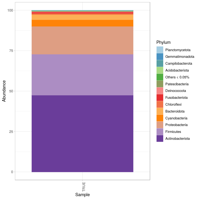
x4 <- tax_glom(metro, taxrank="Phylum")
metrotodos <- c("Pasamanos","Torniquete")
sample_data(x4)$todos = get_variable(x4, "sample_type") %in% metrotodos
mergeph1 <- merge_samples(x4, "todos")
mergeph1
x4 = transform_sample_counts(mergeph1,function(x) (x/sum(x))*100)
data <- psmelt(x4)
head(data)
data$Phylum <- as.character(data$Phylum)
data$Phylum[data$Abundance <= 0.05] <- "Others < 0.05%"
z <- factor(unique(data$Phylum))
z <- nlevels(z)
library(tidyverse)
pd <- data %>%
as_tibble %>%
mutate(Phylum = as.character(Phylum)) # %>%
# replace_na(list(Phylum = "unknown"))
Phylum_abun <- pd %>%
group_by(Phylum) %>%
summarize(Abundance = sum(Abundance)) %>%
arrange(Abundance)
Phylum_levels <- Phylum_abun$Phylum
pd0 <- pd %>%
mutate(Phylum = factor(Phylum, Phylum_levels))
p <- ggplot(pd0, aes(x = Sample, y = Abundance, fill= Phylum, color= Phylum)) + geom_bar(stat = "identity", position="stack") +
scale_fill_manual(values=(colorRampPalette(brewer.pal(10,"Paired"))(z))) +
scale_color_manual(values=(colorRampPalette(brewer.pal(10,"Paired"))(z))) + theme_light() +
theme(axis.text.x=element_text(angle=90, hjust=1)) #+ theme(legend.position="bottom") + guides(fill=guide_legend(nrow=2))
p
ggsave("phylum_allsamples_histogram.pdf")
phyloseq-class experiment-level object
otu_table()   OTU Table:         [ 22673 taxa and 47 samples ]
sample_data() Sample Data:       [ 47 samples by 28 sample variables ]
tax_table()   Taxonomy Table:    [ 22673 taxa by 6 taxonomic ranks ]


phyloseq-class experiment-level object
otu_table()   OTU Table:         [ 40 taxa and 1 samples ]
sample_data() Sample Data:       [ 1 samples by 29 sample variables ]
tax_table()   Taxonomy Table:    [ 40 taxa by 6 taxonomic ranks ]
| <th scope=col>OTU</th><th scope=col>Sample</th><th scope=col>Abundance</th><th scope=col>id</th><th scope=col>sample_location</th><th scope=col>sample_id</th><th scope=col>line_number</th><th scope=col>sample_type</th><th scope=col>date</th><th scope=col>time</th><th scope=col>⋯</th><th scope=col>latitude</th><th scope=col>longitude</th><th scope=col>people_affluence</th><th scope=col>Observed</th><th scope=col>Chao1</th><th scope=col>Shannon</th><th scope=col>Simpson</th><th scope=col>todos</th><th scope=col>Kingdom</th><th scope=col>Phylum</th> | ||||||||||||||||||||
|---|---|---|---|---|---|---|---|---|---|---|---|---|---|---|---|---|---|---|---|---|
| ASV_1 | TRUE | 47.5006996 | 24 | 17.68085 | 24 | 6.297872 | 1.510638 | 3.404255 | 19.85106 | ⋯ | NA | NA | 17859153 | 9903.553 | 15141.15 | 6.380126 | 0.9827077 | 1 | Bacteria | Actinobacteriota |
| ASV_2 | TRUE | 25.3627386 | 24 | 17.68085 | 24 | 6.297872 | 1.510638 | 3.404255 | 19.85106 | ⋯ | NA | NA | 17859153 | 9903.553 | 15141.15 | 6.380126 | 0.9827077 | 1 | Bacteria | Firmicutes |
| ASV_3 | TRUE | 17.2434928 | 24 | 17.68085 | 24 | 6.297872 | 1.510638 | 3.404255 | 19.85106 | ⋯ | NA | NA | 17859153 | 9903.553 | 15141.15 | 6.380126 | 0.9827077 | 1 | Bacteria | Proteobacteria |
| ASV_7 | TRUE | 4.0561480 | 24 | 17.68085 | 24 | 6.297872 | 1.510638 | 3.404255 | 19.85106 | ⋯ | NA | NA | 17859153 | 9903.553 | 15141.15 | 6.380126 | 0.9827077 | 1 | Bacteria | Cyanobacteria |
| ASV_90 | TRUE | 3.1905088 | 24 | 17.68085 | 24 | 6.297872 | 1.510638 | 3.404255 | 19.85106 | ⋯ | NA | NA | 17859153 | 9903.553 | 15141.15 | 6.380126 | 0.9827077 | 1 | Bacteria | Bacteroidota |
| ASV_182 | TRUE | 0.8116411 | 24 | 17.68085 | 24 | 6.297872 | 1.510638 | 3.404255 | 19.85106 | ⋯ | NA | NA | 17859153 | 9903.553 | 15141.15 | 6.380126 | 0.9827077 | 1 | Bacteria | Chloroflexi |
── Attaching packages ─────────────────────────────────────── tidyverse 1.2.1 ──
✔ tibble  2.1.3       ✔ purrr   0.2.5
✔ tidyr   0.8.2       ✔ dplyr   0.8.0.1
✔ readr   1.3.1       ✔ stringr 1.4.0
✔ tibble  2.1.3       ✔ forcats 0.4.0
── Conflicts ────────────────────────────────────────── tidyverse_conflicts() ──
✖ dplyr::filter() masks stats::filter()
✖ dplyr::lag()    masks stats::lag()
Saving 6.67 x 6.67 in image
metro
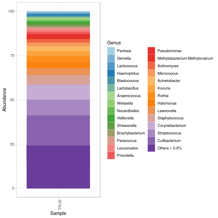
x4 <- tax_glom(metro, taxrank="Genus")
metrotodos <- c("Pasamanos","Torniquete")
sample_data(x4)$todos = get_variable(x4, "sample_type") %in% metrotodos
mergeph1 <- merge_samples(x4, "todos")
mergeph1
x4 = transform_sample_counts(mergeph1,function(x) (x/sum(x))*100)
data <- psmelt(x4)
head(data)
data$Genus <- as.character(data$Genus)
data$Genus[data$Abundance <= 0.5] <- "Others < 0.5%"
z <- factor(unique(data$Genus))
z <- nlevels(z)
z
library(tidyverse)
pd <- data %>%
as_tibble %>%
mutate(Genus = as.character(Genus)) # %>%
# replace_na(list(Phylum = "unknown"))
Genus_abun <- pd %>%
group_by(Genus) %>%
summarize(Abundance = sum(Abundance)) %>%
arrange(Abundance)
Genus_levels <- Genus_abun$Genus
pd0 <- pd %>%
mutate(Genus = factor(Genus, Genus_levels))
p <- ggplot(pd0, aes(x = Sample, y = Abundance, fill= Genus, color= Genus)) + geom_bar(stat = "identity", position="stack") +
scale_fill_manual(values=(colorRampPalette(brewer.pal(10,"Paired"))(z))) +
scale_color_manual(values=(colorRampPalette(brewer.pal(10,"Paired"))(z))) + theme_light() +
theme(axis.text.x=element_text(angle=90, hjust=1)) #+ theme(legend.position="bottom") + guides(fill=guide_legend(nrow=2))
p
ggsave("gemis_allsamples_histogram.pdf")
phyloseq-class experiment-level object
otu_table()   OTU Table:         [ 22673 taxa and 47 samples ]
sample_data() Sample Data:       [ 47 samples by 28 sample variables ]
tax_table()   Taxonomy Table:    [ 22673 taxa by 6 taxonomic ranks ]


phyloseq-class experiment-level object
otu_table()   OTU Table:         [ 1252 taxa and 1 samples ]
sample_data() Sample Data:       [ 1 samples by 29 sample variables ]
tax_table()   Taxonomy Table:    [ 1252 taxa by 6 taxonomic ranks ]
| <th scope=col>OTU</th><th scope=col>Sample</th><th scope=col>Abundance</th><th scope=col>id</th><th scope=col>sample_location</th><th scope=col>sample_id</th><th scope=col>line_number</th><th scope=col>sample_type</th><th scope=col>date</th><th scope=col>time</th><th scope=col>⋯</th><th scope=col>Chao1</th><th scope=col>Shannon</th><th scope=col>Simpson</th><th scope=col>todos</th><th scope=col>Kingdom</th><th scope=col>Phylum</th><th scope=col>Class</th><th scope=col>Order</th><th scope=col>Family</th><th scope=col>Genus</th> | ||||||||||||||||||||
|---|---|---|---|---|---|---|---|---|---|---|---|---|---|---|---|---|---|---|---|---|
| ASV_1 | TRUE | 17.029251 | 24 | 17.68085 | 24 | 6.297872 | 1.510638 | 3.404255 | 19.85106 | ⋯ | 15141.15 | 6.380126 | 0.9827077 | 1 | Bacteria | Actinobacteriota | Actinobacteria | Propionibacteriales | Propionibacteriaceae | Cutibacterium |
| ASV_2 | TRUE | 8.912395 | 24 | 17.68085 | 24 | 6.297872 | 1.510638 | 3.404255 | 19.85106 | ⋯ | 15141.15 | 6.380126 | 0.9827077 | 1 | Bacteria | Firmicutes | Bacilli | Lactobacillales | Streptococcaceae | Streptococcus |
| ASV_6 | TRUE | 8.452160 | 24 | 17.68085 | 24 | 6.297872 | 1.510638 | 3.404255 | 19.85106 | ⋯ | 15141.15 | 6.380126 | 0.9827077 | 1 | Bacteria | Actinobacteriota | Actinobacteria | Corynebacteriales | Corynebacteriaceae | Corynebacterium |
| ASV_5 | TRUE | 5.407315 | 24 | 17.68085 | 24 | 6.297872 | 1.510638 | 3.404255 | 19.85106 | ⋯ | 15141.15 | 6.380126 | 0.9827077 | 1 | Bacteria | Firmicutes | Bacilli | Staphylococcales | Staphylococcaceae | Staphylococcus |
| ASV_4 | TRUE | 4.045221 | 24 | 17.68085 | 24 | 6.297872 | 1.510638 | 3.404255 | 19.85106 | ⋯ | 15141.15 | 6.380126 | 0.9827077 | 1 | Bacteria | Actinobacteriota | Actinobacteria | Corynebacteriales | Corynebacteriaceae | Lawsonella |
| ASV_3 | TRUE | 3.516355 | 24 | 17.68085 | 24 | 6.297872 | 1.510638 | 3.404255 | 19.85106 | ⋯ | 15141.15 | 6.380126 | 0.9827077 | 1 | Bacteria | Proteobacteria | Gammaproteobacteria | Oceanospirillales | Halomonadaceae | Halomonas |
29
Saving 6.67 x 6.67 in image
x4
phyloseq-class experiment-level object
otu_table()   OTU Table:         [ 1252 taxa and 1 samples ]
sample_data() Sample Data:       [ 1 samples by 29 sample variables ]
tax_table()   Taxonomy Table:    [ 1252 taxa by 6 taxonomic ranks ]